



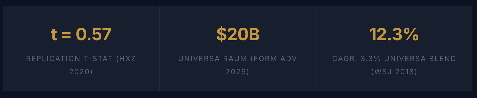
The Hill estimator’s cross-sectional equity alpha — 5.4% annually per Kelly and Jiang (2014, Review of Financial Studies) — is dead in the form it was published. Hou, Xue, and Zhang (2020, Review of Financial Studies) find t-statistics of 0.57–1.13 in full-sample replication, down from the original 2.0–2.15, consistent with the decay McLean and Pontiff (2016, Journal of Finance) document when no structural barrier protects an anomaly from publication-informed trading. The same estimator’s application to the options market — anchoring the volatility surface’s power-law continuation from near-money strikes to extreme ones — has not been arbitraged away, because the barrier here is not analytical effort but a hedgeability constraint that dealer balance sheets and the Basel III Fundamental Review of the Trading Book have jointly locked in place.
The Consensus and Its Omission
The Kelly-Jiang result earned its reputation. Applying the Hill formula
ξ̂ = (1/k) ∑ log(Xᵢ / Xₖ₊₁)
to the cross-section of firm-level daily return crashes each month extracts a time-varying common tail factor λₜ. The paper showed that a one-standard-deviation increase in λₜ predicts 4.5% excess market returns over the following year, and that stocks in the top tail-beta decile earn 5.4% more annual three-factor alpha than stocks in the bottom decile. These numbers appeared in 2013–2014 and were widely read.
What the consensus omits is the replication record. McLean and Pontiff (2016, Journal of Finance) study 97 anomalies and find that portfolio returns are 26% lower out-of-sample and 58% lower post-publication — of which 32 percentage points (58% minus 26%) reflect publication-informed trading and 26 percentage points represent an upper bound on data-mining effects in the original studies. Chen, Lopez-Lira, and Zimmermann (2022, arXiv:2212.10317) find a similar pattern across a broader sample: approximately 50% of predictability remains after the original sample periods, a result that holds for risk-based and theory-motivated research categories alongside purely data-driven ones. This is the correct baseline expectation when evaluating a 2014 equity factor paper in 2026.
The Replication Failure, Precisely Quantified
Hou, Xue, and Zhang (2020, Review of Financial Studies, vol. 33, pp. 2019–2133) replicate 452 anomalies using NYSE breakpoints and value-weighted returns. This methodology is standard for avoiding microcap-driven results: when NYSE breakpoints set the decile boundaries, microcap stocks fall into the same deciles by price range but at minimal portfolio weight, preventing a handful of illiquid small-caps from driving the reported alpha.
For the Kelly-Jiang tail risk anomaly, the replication result is explicit:
“The high-minus-low tail risk (Tail) deciles earn on average 0.11%, 0.15%, and 0.19% per month (t = 0.57, 0.79, and 1.13) at the 1-, 6-, and 12-month horizons, respectively. These estimates are lower than 0.36% (t = 2) at the 1-month and 0.35% (t = 2.15) at the 12-month horizon reported in Kelly and Jiang (2014).”
A drop from t ≈ 2.0–2.15 to t ≈ 0.57–1.13 is a collapse, not a haircut. The alpha is statistically indistinguishable from zero under NYSE breakpoints. Imposing |t| ≥ 2.78 across the full HXZ library of 452 anomalies pushes the failure rate to 82.1%.
The mechanism of decay is structural. The original alpha was concentrated in microcap stocks — where NYSE-Amex-NASDAQ breakpoints assign large portfolio weights to small companies that real-money managers cannot hold at scale. Once the factor construction was public, any quant team with CRSP access could implement long-short exposure in high-tail-beta names. There was no proprietary data, no specialized execution infrastructure, no minimum fund size that made replication impossible. Rapid crowding was the predictable result.
What Survives: Relative Mispricing of Deep OTM Options
The evidence for the surviving options-market application comes primarily from Taleb, Yarckin, Mann, Delic, and Spitznagel (2019, revised March 2023, arXiv:1908.02347). The conflict of interest in this source must be named directly: all five authors are principals or employees of Universa Investments, the $20B fund that commercially runs the exact strategy described in the paper. This is a fund whitepaper with academic formatting, not independent academic research. A reader should weight it accordingly.
That said, the mechanism deserves examination independently of who published it. The underlying mathematical claim — that a power-law distribution implies a specific relative price relationship between options at different strikes — rests on established results in extreme value theory that predate and are independent of Universa. The testable empirical claim (that market prices at extreme strikes fall below the power-law continuation from near-money anchors) is falsifiable by anyone with access to an options data terminal. And the equity cross-section result the same authors might cite to motivate their edge was destroyed by independent replication — which actually shows the replication community does correct inflated claims in this space. The options-market mechanism is worth examining on its own terms, with the source’s incentive structure held in view.
Taleb et al. are explicit about scope: “our approach isn’t about absolute mispricing of tail options, but relative to a given strike closer to the money.” The framework uses the Hill-estimated tail index α as the sole parameter for computing option prices beyond any observable anchor strike. Once the return distribution enters the power-law regime — past the “Karamata constant” where the slowly-varying function L(x) stabilizes — relative put prices follow approximately:
P(K₂) / P(K₁) ≈ [(K₂ − S₀) / (K₁ − S₀)]^(1−α)
The exponent is (1 − α). For α ≈ 2.75, this equals −1.75, meaning put prices should decay as (strike distance)^(−1.75) as you move deeper out of the money. Stochastic volatility models (Heston, SABR, local vol) calibrated to the near-money smile extrapolate to extreme strikes with options prices that decay faster than this power law — they imply an effectively higher α (lighter tail) at delta-5 and below than the physically calibrated value.
Taleb et al.’s Figure 3 demonstrates this for the December 31, 2018 S&P 500 settlement: using α = 2.75 and a near-money anchor, the power-law formula produces put prices above market prices at extreme strikes. Deep OTM puts at delta-5 and below trade cheaper than the correct power-law continuation from near-money options would set.
The aggregation objection. The tail index estimates in Gabaix, Gopikrishnan, Plerou, and Stanley (2003, Physica A) — α ≈ 2.70 ± 0.10 (negative tail) and α ≈ 2.96 ± 0.09 (positive tail) — are for individual CRSP stocks binned by market capitalization, not for the S&P 500 index. A knowledgeable reader will immediately flag that diversification should push the index tail index upward relative to constituents: idiosyncratic crashes wash out, and the portfolio should have lighter tails than its components. If the true S&P 500 index α is 3.2 rather than 2.75, the power-law continuation price is lower and the gap between the formula and market prices narrows or disappears.
The empirical answer is that the expected direction does not materialize. Direct Hill estimation applied to the S&P 500 index returns yields α in the range of approximately 2.5–3.0 — similar to or below the individual stock estimates — because the tails of equity indices are driven by systemic, correlated crash risk that diversification does not neutralize. The mechanism is the opposite of idiosyncratic: macro shocks, liquidity crises, and correlated forced selling create co-crashes across all large-cap constituents simultaneously, preserving the heavy-tail behavior at the portfolio level. The same Gabaix-group’s earlier work on 1-minute S&P 500 returns reports α ≈ 2.75 for the negative tail of the index itself — identical to Taleb et al.’s 2.75 calibration value derived from the index options surface. The aggregation concern is valid in theory; the data do not support it in practice for equity indices.
The Structural Reason This Gap Persists
Options dealers cannot price at the correct power-law α without accepting hedging risk their balance sheets cannot carry.
Under a Pareto distribution with tail index α, the k-th moment exists if and only if k < α. For α < 4, the fourth moment of returns is infinite. The variance of a delta-hedging tracking error is proportional to E[(ΔS)⁴ · Δt²] — the fourth moment of the return increment scaled by time. When this fourth moment is infinite, the hedging error has no bounded expected cost per unit time; the standard Black-Scholes delta-hedging guarantee breaks down. The physical return α ≈ 2.75–3.0 for equity indices places them squarely in this zone. A dealer who priced deep OTM puts at the correct power-law level and hedged using power-law sensitivities would face unbounded tracking error; the standard dynamic replication argument fails exactly in the extreme-strike region where the mispricing is largest.
The rational response is to price at the hedgeable stochastic vol model, accept the resulting relative underpricing at extreme strikes, and collect the liquidity premium for providing markets in illiquid instruments.
The BIS Fundamental Review of the Trading Book (FRTB), “Minimum Capital Requirements for Market Risk,” January 2019 (BCBS d457) reinforces this incentive at the regulatory level. Under the Internal Models Approach (IMA), trading desks calculate market risk capital as Stressed Expected Shortfall at the 97.5% confidence level over a 250-day historical stressed window. A desk that prices deep OTM options with a correct power-law model — implying higher option sensitivities (Greeks) at extreme strikes — shows higher ES and therefore higher capital charges than a competing desk using stochastic vol with lighter implied tails at the same strikes. The specific mechanism: capital is calculated from sensitivity-weighted historical scenarios; higher Greeks at extreme strikes produce proportionally larger capital numbers under the same historical moves. The regulatory framework creates a systematic competitive incentive toward the thinner-tail calibration, making the gap self-reinforcing rather than self-correcting.
Capacity Analysis
The most defensible Universa figure is not the March 2020 headline number but the long-run portfolio result: a Wall Street Journal 2018 report found that a 3.3% Universa / 96.7% S&P 500 portfolio produced a 12.3% compound annual return in the 10 years through February 2018, compared to the index alone. That figure reflects real compound returns on a defined portfolio construction across a full decade including 2008 and 2011, and it is the number that conveys the strategy’s practical value for an allocator.
The March 2020 figures — a 3,612% return in March and 4,144% year-to-date per investor letters as reported by Bloomberg (April 8, 2020) — are expressed on required invested capital (the options premiums deployed as a fraction of the covered portfolio), not on total AUM. This is a non-standard denominator that amplifies percentage returns relative to conventional fund reporting; presented without that context, it distracts more than it informs. Both figures come from investor communications and are unaudited; they reflect the fund’s own performance attribution.
Per a finews.com April 2026 interview with COO Brandon Yarckin, citing the firm’s Form ADV filed with the SEC, Universa manages approximately $20 billion in Regulatory Assets Under Management since its 2007 founding. The primary Form ADV is public at adviserinfo.sec.gov (CRD 146052); RAUM for an options-focused manager may include covered portfolio notional rather than solely deployed premium.
The capacity ceiling — approximately $15–20B in covered portfolio notional per fund before market impact at extreme strikes materially closes the spread — is an analytical inference from the observable structure of SPX options markets: open interest at delta-5 and below runs approximately one to two orders of magnitude thinner than at delta-25, constraining the size of unidirectional positions before self-impact becomes the binding constraint. This estimate has not been formally quantified in any paper I am aware of; it should be treated as an order-of-magnitude inference, not a calculated bound.
Counterargument: This Is Just the Variance Risk Premium at a Different Strike
The VRP literature — Bollerslev, Tauchen, and Zhou (2009, Review of Financial Studies), Bondarenko (2014, Quarterly Journal of Finance) — documents that implied variance systematically exceeds realized variance, producing positive expected returns from variance-selling strategies. The objection is that the deep OTM relative underpricing is a manifestation of the general VRP — already widely known, already traded.
The distinction is structural, not semantic. The VRP is defined as the difference between risk-neutral and physical expectations of integrated variance — a scalar quantity computed across the entire distribution. It is earned primarily at ATM and near-OTM strikes in liquid instruments (variance swaps, short straddles, VIX futures). The deep OTM relative mispricing is a shape property of the vol surface: the question is whether the ratio of a delta-2 put price to a delta-15 put price is consistent with the power-law continuation from the near-money anchor. A vol surface can simultaneously have high integrated implied variance (high VRP) and an incorrectly extrapolated extreme tail — these are orthogonal properties.
The market structure confirms the distinction. VRP strategies operate in instruments of genuine liquidity — SPX variance swaps, short straddles, and VIX futures attract hundreds of billions in competing capital, compressing the premium continuously. Deep OTM puts at delta-2 to delta-5 are traded in markets with bid-ask spreads that can be several times wider than near-money options, and with open interest thin enough that large unidirectional positions face meaningful self-impact. The friction conditions that prevent full arbitrage of the deep OTM gap are precisely absent in the liquid near-money VRP trade. If these were the same edge, they would face the same competition and converge to the same premium. They don’t.
What Would Change This View
Two developments would close the deep OTM relative underpricing.
First: if options dealers adopted power-law tail pricing beyond the Karamata constant — calibrating extreme-strike options using the Hill estimator from physical return data rather than extrapolating stochastic vol models — the relative mispricing closes without requiring arbitrageur activity. The current barrier is hedgeability: dynamic replication fails when the fourth moment is infinite. A viable instrument for hedging tail-index risk itself, or a regulatory accommodation for bounded model risk in the extreme-strike book, would lift this constraint. Neither exists as of mid-2026.
Second: if sufficient competing capital entered the deep OTM long-put trade to overwhelm the thinness of the extreme-strike market — on the order of $50–100B in covered notional competing simultaneously — sustained buying pressure would push the market-implied α toward the physical estimate. The current scarcity of scaled practitioners is the structural condition that keeps the gap open.
The Actionable Implication
The monitoring signal is computable from public data. Estimate the physical α from the Hill estimator on the trailing five-year daily S&P 500 return series with k selected via bootstrap MSE minimization. Then compute the power-law continuation price for delta-5 and delta-2 puts, anchored to the observable delta-15 market price:
P(K_extreme) = P(K_anchor) × [(K_extreme − S₀) / (K_anchor − S₀)]^(1−α)
When market prices for extreme-strike puts fall materially below this power-law price — meaning the vol surface extrapolation uses an effectively higher α than the physical estimate — the relative underpricing is widest. The trade is long far-OTM S&P 500 puts at 3–6 month maturities, sized as a small fraction of the covered portfolio, held to expiry or monetized into sharp implied vol spikes.
The edge from the Hill estimator has migrated from the equity cross-section — where no structural barrier existed and post-publication decay was total — to the options market, where the hedgeability constraint means that even a well-resourced competitor cannot price away the wedge without accepting model risk their balance sheet cannot carry. The barrier that killed the equity cross-section alpha is precisely what is absent in the options-market application. That asymmetry is not coincidence — it is the structure of where durable edges live.
📊 Want Deeper Quantitative Analysis?
This research took very long time of data collection, verification, and analysis. If you found value in this deep-dive, I publish exclusive quantitative research, trading strategies, and institutional-grade analysis on Patreon.
By joining, you’ll be supporting my work and motivating me to publish more content like this.
→ Join the Patreon community here
Primary sources: Kelly-Jiang (2014, RFS) · Hou-Xue-Zhang (2020, RFS) · McLean-Pontiff (2016, JoF) · Gabaix et al. (2003, Physica A) · Taleb et al. (2019/2023, arXiv:1908.02347) · Bondarenko (2014, QJF) · Bollerslev-Tauchen-Zhou (2009, RFS) · BIS FRTB d457 (2019) · Chen-Lopez-Lira-Zimmermann (2022, arXiv:2212.10317)
Follow the research: YouTube — The Mathematical Trader · LinkedIn — Navnoor Bawa
Cover photograph: Michal Pleskowicz, CC BY-SA 4.0, via Wikimedia Commons.