



The Gambler’s Delusion That Wall Street Couldn’t Resist
On October 27, 1997, Victor Niederhoffer — then ranked the world’s #1 hedge fund manager with 15 years of 35% annualized returns — watched his $130 million fund evaporate to zero in a single trading session. By 4 PM, Niederhoffer had lost everything: his clients’ capital, his personal fortune, even the antique silver collection he’d later auction to cover margin calls.
His mistake wasn’t complex. It was mathematically elementary.
Niederhoffer had sold thousands of S&P 500 put options — effectively selling insurance against a market crash — collecting small premiums while betting the market wouldn’t drop significantly. When the Dow plunged 554 points that Monday, he didn’t just lose money. He lost the ability to continue playing the game. His broker issued a margin call he couldn’t meet. The strategy that had worked hundreds of times before failed catastrophically on attempt number 101.
This is the Martingale Paradox: a betting strategy that appears mathematically sound in theory but guaranteed to fail in practice due to constraints that always exist in real markets.
What Is the Martingale Strategy?
The Martingale system originated in 18th-century France as a betting strategy for games with near 50/50 odds. The logic is seductive:
Bet $1 on a coin flip
If you lose, double your bet to $2
If you lose again, double to $4, then $8, then $16
When you eventually win, you recover all previous losses plus a $1 profit
Reset and repeat
Mathematically, if you have infinite capital and no betting limits, this strategy is certain to profit. You will eventually flip heads. The question is never “if,” only “when.”
In financial markets, the analog is equally tempting: Sell insurance against unlikely events. Collect small, consistent premiums. Double down when markets move against you. Eventually, markets revert to normal, and you profit.
The Mathematical Guarantee That Doesn’t Guarantee Anything
The formal mathematics supporting Martingale strategies come from martingale probability theory, developed by French mathematician Paul Lévy in 1934. A martingale is a stochastic process where the expected future value, given all past information, equals the current value — a “fair game” in mathematical terms.
The critical insight: The Optional Stopping Theorem proves that betting strategies cannot change the expected value of fair games. If a game has zero expected value (neither player has an edge), no betting strategy — including Martingale — can create positive expected value.
This creates an immediate mathematical problem. Consider a simple Martingale on an unfavorable game like roulette (house edge of 5.26%):
Expected value per round:
Probability of 6 consecutive losses: (10/19)⁶ = 2.13%
Probability of winning within 6 rounds: 97.87%
Expected gain: 1 × 0.9787 = 0.9787
Expected loss: 63 × 0.0213 = 1.3419
Net expected value: -0.363 per cycle
The Martingale doesn’t eliminate the house edge. It redistributes outcomes: you win small amounts frequently (97.87% of the time) and lose catastrophically rarely (2.13% of the time). The expected value remains negative, but the distribution of outcomes fundamentally changes.
This distribution change creates a psychological trap. Traders experience repeated small wins — Niederhoffer made profits on his put-selling strategy for months — which reinforces the behavior. Then a tail event occurs, and accumulated gains evaporate instantly.
The Real-World Constraints That Guarantee Failure
In theory, Martingale works with three conditions:
Infinite wealth
No betting limits
Infinite time horizon
In practice, all three conditions are always violated:
Constraint 1: Capital Is Finite
The geometric growth of position sizes creates exponential capital requirements. Starting with a $10,000 position:
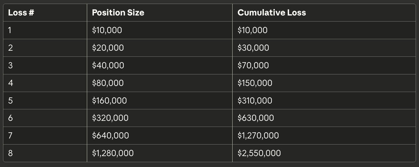
After just 8 consecutive losses — an event with probability 1/256 for a 50/50 game — you need $2.55 million in capital to continue. After 10 losses (probability 1/1,024), you need over $10 million.
Real-world example: Victor Niederhoffer had $130 million in assets. After losing approximately $50 million on Thai bank positions in July-August 1997, his remaining capital couldn’t sustain the position sizes required when the S&P 500 dropped 7.2% on October 27. His 830 S&P put options required margin he no longer had. He was forced to liquidate at the worst possible time.
The cruel irony: By November 1997, the S&P 500 had recovered, and Niederhoffer’s put options expired worthless. His trade would have been profitable — if he’d survived October 27. Capital constraints forced exit at maximum loss.
Constraint 2: Position Limits Exist
Even if capital were available, exchanges and brokers impose position limits. No institution allows unlimited position sizing. When markets move against leveraged positions, brokers issue margin calls that must be met within hours — not days or weeks.
Constraint 3: Time Horizons Are Finite
Markets can remain irrational longer than you can remain solvent. The most sophisticated hedge fund in history learned this lesson the hard way.
Case Study 1: Long-Term Capital Management — When Genius Isn’t Enough
The Nobel Prize-Winning Disaster
Long-Term Capital Management (LTCM) was founded in 1994 by John Meriwether, former vice-chairman of Salomon Brothers, alongside Nobel laureates Myron Scholes and Robert Merton — the architects of the Black-Scholes options pricing model. If anyone understood the mathematics of risk, it should have been them.
LTCM’s strategy was sophisticated but fundamentally Martingale-like:
Identify pricing inefficiencies between similar securities
Buy undervalued bonds, short overvalued bonds
Collect small spreads as prices converge
Use massive leverage to amplify tiny edges
The results were initially spectacular:
1994: +21% returns (after fees)
1995: +43% returns
1996: +41% returns
1997: +17% returns (down from prior years, signaling strategy decay)
By 1998, LTCM managed $4.7 billion in equity but controlled:
$125 billion in borrowed capital
$1.25 trillion in derivatives (notional value)
Effective leverage ratio: 250:1 by September 1998
The Fatal Martingale Elements
LTCM’s convergence trades were fundamentally Martingale bets:
Trade Structure: Buy 30-year off-the-run Treasury bonds (undervalued), short 30-year on-the-run Treasury bonds (overvalued). Spreads between these nearly identical securities should converge to zero within months.
The Problem: Spreads can diverge before they converge. When Russia defaulted on its debt in August 1998, investors fled to the safest assets — on-the-run Treasuries — causing spreads to widen dramatically. LTCM’s “sure thing” positions moved against them.
The Martingale Response: Instead of cutting losses, LTCM increased position sizes. When initial bets failed, they doubled down, assuming markets would eventually revert. They were playing a perfect Martingale.
How The Money Was Lost
In August 1998 alone, LTCM lost $1.9 billion — 44% of capital. By September, the fund was hemorrhaging:
Specific losses:
Russian and emerging market positions: Lost $430 million when Russia defaulted and currency hedges failed (Russian government prevented further trading)
Interest rate swaps: Lost $1.6 billion as credit spreads widened instead of narrowing
Equity volatility: Lost money shorting S&P 500 options as volatility spiked
Equity pairs trading: Lost $286 million as correlations broke down
The leverage multiplier: With 250:1 effective leverage, a 2% move against LTCM became a 500% loss relative to equity. In a single month, positions that were “4 standard deviations unlikely to fail” actually failed.
On September 23, 1998, the Federal Reserve orchestrated a $3.625 billion bailout from 14 major banks — not to save LTCM’s partners, but to prevent a systemic financial crisis. LTCM’s positions were so large and so levered that forced liquidation would have destabilized global markets.
LTCM’s equity value on rescue: $400 million (down from $4.7 billion in January)
Lessons:
Leverage converts small losses into catastrophic ones
“Impossible” events happen with disturbing regularity
Time horizon matters: LTCM’s models assumed they could wait out adverse moves. Margin calls disagreed.
Even perfect mathematics cannot overcome capital constraints
Case Study 2: Victor Niederhoffer — Pride Before The Fall
From George Soros’s Star Trader to Bankruptcy
Victor Niederhoffer wasn’t some reckless gambler. He was:
Harvard-educated statistician with a PhD in economics
Five-time U.S. squash champion (discipline personified)
Former partner to George Soros
Author of a bestselling book on speculation
Ranked #1 hedge fund manager in 1996 by MAR
In his own words, Niederhoffer claimed his trading success was “700 standard deviations away from randomness” — essentially arguing his edge was mathematically certain.
The Setup: How To Lose $130 Million in One Day
Summer 1997: The Thai Bank Fiasco
Niederhoffer noticed Thai bank stocks had fallen dramatically during the Asian Financial Crisis. Based partly on a friend’s observation that Bangkok’s red-light district looked “cleaner and safer” — a dubious indicator of economic recovery — Niederhoffer placed large bets on Thai banks and the baht currency.
When Thailand abandoned its currency peg on July 2, 1997, the baht crashed more than 17% in a single day. Niederhoffer lost approximately $50 million — nearly 40% of his fund’s assets.
August-September 1997: The Martingale Doubling Down
Rather than accepting the loss and reducing risk, Niederhoffer engaged in classic Martingale behavior: he tried to “get even” by selling massive quantities of S&P 500 put options.
The Trade:
Sold approximately 1,000 November 830 S&P put options
Collected $4–6 per contract in premiums (total: ~$5 million in premiums)
S&P 500 was trading around 950
Options would expire worthless if S&P stayed above 830 by November
The Math: Niederhoffer was selling insurance against an S&P drop below 830 — approximately a 12% decline. Historical volatility suggested this was unlikely in a 60-day window. Each day the market stayed calm, Niederhoffer collected option premium decay.
This is the Martingale trap: High probability of small gains (collecting premiums), low probability of catastrophic loss (payout if market crashes).
October 27, 1997: The Day Everything Failed
The Asian Financial Crisis spread to Hong Kong. On October 27, 1997:
7:00 AM ET: Hong Kong’s Hang Seng Index opens sharply lower
9:30 AM ET: Dow Jones opens down 200 points
By 2:00 PM ET: Dow is down 554 points (-7.2%) — the 8th largest point decline in history
3:30 PM ET: S&P 500 futures trigger exchange circuit breakers
4:00 PM ET: Markets close. Niederhoffer’s put options are suddenly deep in-the-money
The P&L Mechanics:
When S&P dropped from 950 to 876 (closing price), Niederhoffer’s 830 put options increased in value exponentially due to two factors:
Intrinsic value change: Minimal (still out-of-the-money)
Implied volatility explosion: VIX-equivalent measures spiked 100%+
Put option value = Intrinsic Value + Time Value + Volatility Premium
The volatility spike alone caused options Niederhoffer sold for $4–6 to trade at $15–20. On 1,000 contracts (each representing 500 shares of S&P exposure), this was approximately:
Options sold for: $5 million (premium collected)
Current mark-to-market value: $20 million+ (cost to buy back)
Unrealized loss on options alone: -$15 million
Margin requirement: $50–70 million (to maintain short option positions)
When his broker Refco demanded additional margin, Niederhoffer couldn’t post it. Refco began liquidating his positions at 3:45 PM — 15 minutes before market close, at the absolute worst prices of the day.
Total losses on October 27: Approximately $130 million
What Happened Next
Niederhoffer declared bankruptcy
Auctioned his antique silver collection and rare books
Mortgaged his Connecticut mansion
Filed a lawsuit against the Chicago Mercantile Exchange (lost)
The Bitter Irony:
By November 1997, the S&P 500 recovered to 955. Niederhoffer’s November 830 puts expired worthless — exactly as his model predicted. His trade was fundamentally correct. But capital constraints forced liquidation at maximum loss.
In Niederhoffer’s own words (Washington Post, November 17, 1997):
“I’ve made that trade hundreds of times in the past 15 years. I was a victim of circumstances I could not have foreseen.”
This is the Martingale delusion. The strategy works hundreds of times — until the one time it doesn’t. And that one failure erases all previous gains.
The Second Blow-Up: 2007
Remarkably, Niederhoffer rebuilt his fund. By 2006, he was running the Matador Fund with strong performance. Then came the 2007 subprime mortgage crisis. Using similar volatility-selling strategies, Niederhoffer lost 75% of the fund’s value in a single quarter.
Pattern recognition: Same trader. Same strategy. Different crisis. Same result.
Case Study 3: The XIV Collapse — When Retail Investors Learned About Tail Risk
The “Free Money” Machine (2012–2018)
By 2012, a new generation of traders discovered what they thought was a foolproof strategy: shorting volatility through leveraged ETFs.
The Product: Credit Suisse VelocityShares Daily Inverse VIX Short-Term ETN (ticker: XIV)
What it did:
Provided inverse exposure to VIX futures
When VIX went down 1%, XIV went up 1%
Rebalanced daily to maintain constant short exposure
Why people loved it:
From 2012–2017, XIV generated spectacular returns:
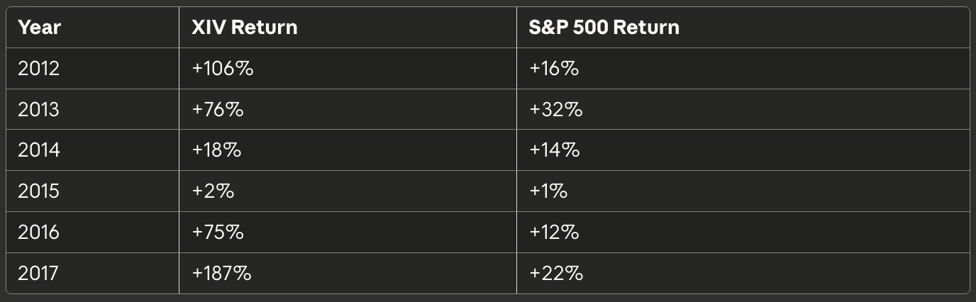
Cumulative 2012–2017: XIV returned 565% vs. S&P 500’s 86%
This created a feedback loop:
Investors see amazing returns
More money flows into XIV
Short volatility positions grow larger
Volatility gets suppressed further (self-reinforcing)
Returns look even better
Repeat
By January 2018, XIV had $2 billion in assets. Combined with similar products like SVXY, over $4 billion was betting against volatility spikes.
The Fatal Flaw: Volatility of Volatility
XIV worked perfectly when markets were calm. But it had a hidden Martingale structure:
Daily P&L formula: Daily Return = -(Previous Day VIX Return) × Leverage
This meant:
VIX drops 1% → XIV gains 1% (small, consistent wins)
VIX spikes 100% → XIV loses 100% (total wipeout)
The product prospectus disclosed this risk clearly: “An acceleration event occurs if the ETN loses more than 80% of its value in a single day.”
Acceleration event = automatic liquidation = investors lose everything.
February 5, 2018: Volmageddon
The Trigger: U.S. wage growth data came in higher than expected, raising inflation fears and interest rate hike expectations. Markets began selling off.
The Cascade:
9:30 AM ET: S&P 500 opens lower, VIX rises from 18 to 20
12:00 PM ET: Selling intensifies, VIX hits 25
2:00 PM ET: S&P 500 down 2%, VIX at 30
3:00 PM ET: Volatility products begin rebalancing (must buy VIX futures to maintain hedge ratios)
3:30 PM ET: Forced buying of VIX futures creates feedback loop
4:00 PM ET: VIX closes at 37.32 (+115% in one day — largest single-day VIX spike on record)
After-hours trading (4:00–8:00 PM):
This is when the real carnage occurred. XIV and similar products had to rebalance their portfolios based on the 4 PM closing prices. This meant buying billions of dollars of VIX futures in thin after-hours markets.
The death spiral:
XIV drops 15% during regular hours
After-hours rebalancing forces VIX futures buying
Buying pushes VIX futures higher
Higher VIX futures cause XIV to drop further
Further drops require more rebalancing
More buying pushes VIX futures even higher
Acceleration event triggered at 80% loss threshold
Final damage:
XIV: Closed February 2 at $115.73 → After hours February 5: $4.22 (-96%)
SVXY: Closed February 2 at $103.72 → After hours February 5: $3.96 (-96%)
Credit Suisse announced the termination of XIV on February 6, 2018. The last trading day was February 20, 2018. Investors received approximately $5 per share based on the closing indicative value — a 95% loss from the all-time high just weeks earlier.
Who Lost Money?
Known casualties:
Retail investors who treated XIV as a “conservative income strategy”
A Reddit user documented losing $4 million in a single day
Hedge funds including exposures from Citadel Advisors, Deutsche Asset Management, and Two Sigma (though exact losses undisclosed)
Total investor losses: Estimated at $3–4 billion across all short volatility products during the February 2018 event.
The Martingale Connection
XIV investors were executing a textbook Martingale:
Small, consistent premiums (VIX decay from contango)
Held positions too large for their capital base
Assumed “impossible” events (80% single-day loss) wouldn’t occur
No exit plan when tail events materialized
The mathematics that made XIV attractive (expected value positive from VIX term structure) were correct. But the fat-tailed risk distribution made the strategy unplayable at scale.
The Mathematical Proof of Why Martingale Always Fails
The Optional Stopping Theorem
The formal proof that Martingale strategies cannot beat negative expectancy games comes from the Optional Stopping Theorem, first rigorously proven by Joseph Doob in the 1950s.
Theorem Statement:
Let X be a martingale (fair game) with respect to filtration F, and let T be a stopping time. Then under certain conditions:
E[X_T] = E[X_0]
In plain English: Your expected wealth when you stop playing equals your expected wealth when you started. No betting strategy can change this.
The Three Conditions:
The theorem holds if ANY of the following is true:
T ≤ N (bounded stopping time): You must stop after N rounds maximum
|X_n| ≤ K (bounded stakes): Your bets cannot exceed K dollars
E[T] < ∞ and increments bounded: Expected stopping time is finite and bet sizes are bounded
Why This Destroys Martingale:
Real-world trading satisfies ALL three conditions:
Bounded time: You don’t have infinite years to trade. Margin calls arrive in days or hours.
Bounded stakes: Exchanges and brokers impose position limits. You cannot place infinite-sized bets.
Finite stopping time: Bankruptcy, margin calls, or risk limits force exit.
The Gambler’s Ruin Problem
The classic illustration of Martingale failure:
Setup: Gambler starts with $100. Betting $1 per round on a fair coin flip. Doubles bet after losses. Stops when reaching $200 (target) or $0 (bankrupt).
Question: What’s the probability of reaching $200 before going bankrupt?
Answer: Exactly 50% (for a fair game)
Expected number of rounds: 10,000
The Martingale doesn’t improve your odds. It just changes the distribution of outcomes:
50% of the time: Slow, steady progress to $200
50% of the time: Catastrophic wipeout to $0
The “slow and steady” appearance creates the illusion of a winning system. But the expected value remains zero.
Why Capital Requirements Explode
The probability of K consecutive losses in a fair game is:
P(K losses) = (1/2)^K
The capital required to sustain K losses is:
Capital(K) = Initial_Bet × (2^(K+1) — 1)
This creates exponential capital requirements:
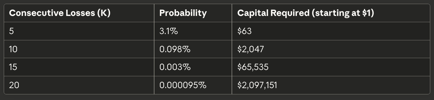
Even seemingly “impossible” events (20 consecutive losses = 1 in 1,048,576) require only $2.1 million in capital to survive. But how many traders have $2.1 million available for a single $1 bet?
The mathematical certainty: Given enough trials, you WILL experience a streak that exceeds your capital base. It’s not “if,” it’s “when.”
Why Smart People Keep Falling For It
The Psychological Trap
Martingale strategies create powerful psychological reinforcement:
1. Frequent Small Wins
You experience winning 95%+ of the time. This creates:
Confirmation bias (the strategy “works”)
Overconfidence (you’re “good at trading”)
Recency bias (recent wins overshadow theoretical tail risk)
Victor Niederhoffer made money for 180 consecutive months before October 1997. LTCM had four years of spectacular returns. XIV investors watched their accounts compound for five years straight.
2. Apparent Control
Unlike pure gambling, trading involves:
Complex models (creates illusion of edge)
Market analysis (feels like skill-based activity)
Historical backtests (shows strategy “worked” in the past)
This obscures the fundamental truth: You’re selling insurance against rare events without sufficient capital to pay claims when they arrive.
3. Survivorship Bias
Successful Martingale traders are celebrated. Failed ones disappear. Before Niederhoffer’s collapse, he was the #1 hedge fund manager. Before LTCM failed, its partners won Nobel Prizes. Before XIV imploded, it was the fastest-growing ETF.
The graveyard of failed Martingale traders is large and silent. The few survivors (so far) are loud and visible.
The Taleb Critique
Nassim Nicholas Taleb, author of The Black Swan, visited Victor Niederhoffer’s office in 1996 — one year before the collapse. His observation:
“The strategy amounts to selling flood insurance. Most years you collect premiums and look brilliant. Then comes a hurricane, and you’re bankrupt.”
Taleb noted that Niederhoffer had converted positive skewness (many small losses, rare large wins — like buying insurance) into negative skewness (many small wins, rare catastrophic losses — like selling insurance).
The expected value can be identical, but the lived experience is radically different:
Strategy A (Buying Options):
Lose $1 per day for 99 days
Win $200 on day 100
Net: +$101 over 100 days
Experience: Feels like bleeding money with rare jackpots
Strategy B (Selling Options — Martingale):
Win $2 per day for 99 days
Lose $200 on day 100
Net: +$101 over 100 days (same expected value)
Experience: Feels like printing money until sudden catastrophe
Strategy B attracts more traders because it feels good psychologically. But the math is identical — and the practical risk is worse because loss arrives as a concentrated shock rather than distributed over time.
Modern Incarnations: Where Martingale Hides Today
1. “Volatility Harvesting” Strategies
What they are: Systematically selling options to collect premium, often with “dynamic hedging.”
Why it’s Martingale: Small consistent gains from option decay, occasional catastrophic losses from volatility spikes.
Who uses them: Volatility arbitrage funds, covered call ETFs (e.g., JEPI, XYLD), short premium trading systems.
2. Risk Parity Funds
What they are: Leverage low-volatility assets (bonds) to match the risk of high-volatility assets (stocks).
Why it’s Martingale: Works beautifully when volatility is stable and mean-reverting. Fails catastrophically when volatility regimes shift (March 2020, 2022).
Who uses them: Bridgewater Associates (though sophisticated), retail “all-weather portfolios.”
3. Algorithmic “Grid Trading”
What it is: Place buy orders at progressively lower prices, selling when price rebounds.
Why it’s Martingale: Averages down into losing positions, assuming price will eventually recover.
Who uses it: Crypto traders, forex robots, retail algorithmic traders.
4. Leveraged ETFs Held Long-Term
What they are: 2x or 3x leveraged ETFs designed for daily trading, held for months or years.
Why it’s Martingale: Volatility decay erodes value even when underlying moves favorably. Investors who “buy the dip” are doubling down on losing positions.
Who uses them: Retail investors who don’t understand daily rebalancing mechanics.
The Three Lessons Professional Traders Actually Learn
Lesson 1: Position Sizing Is Everything
The mathematically optimal bet size for a positive-expectancy strategy is given by the Kelly Criterion:
f = (bp — q) / b*
Where:
f* = fraction of capital to bet
b = odds received on bet
p = probability of winning
q = probability of losing (1 — p)
For Martingale-style strategies with negative skew:
Never bet more than 0.5–1% of capital per trade
Stop loss MUST be defined before entering
Maximum drawdown tolerance must be set before first trade
Niederhoffer violated this by betting 40% of his capital on Thai banks, then tried to recover by betting 60% on S&P puts. LTCM violated this with 250:1 leverage.
Lesson 2: Time Horizon Matters More Than Expected Value
LTCM’s convergence trades had positive expected value. Given infinite time, spreads would converge. But margin calls arrive in days, not years.
Practical rule: Your time horizon must exceed the maximum drawdown duration by at least 3x.
If your strategy can experience 6-month drawdowns, you need 18+ months of capital to survive. If you’re levered, you need even more.
Lesson 3: Tail Events Are Not “Black Swans” — They’re Inevitable
The October 1987 crash was “25 standard deviations impossible.” It happened.
The 1998 Russian default was “never supposed to happen.” It happened.
The 2008 financial crisis violated “all models.” It happened.
The March 2020 COVID crash came “out of nowhere.” It happened.
The February 2018 VIX spike was “physically impossible.” It happened.
Pattern: Every Martingale failure is preceded by the belief that “this time is different” or “that event is too unlikely to matter.”
Reality: Fat-tailed distributions mean tail events occur with frequency orders of magnitude higher than normal distributions predict. Nassim Taleb calls this “Mediocristan vs. Extremistan.”
Practical implication: If your strategy cannot survive a 6-sigma event, you’re playing Russian roulette with enough cylinders that you’ll eventually hit the bullet.
What Actually Works: Anti-Martingale Position Sizing
The opposite of Martingale — increasing position size when winning, decreasing when losing — has robust mathematical support.
Why Anti-Martingale Works:
Preserves capital during drawdowns: Small bets when equity curve is declining
Capitalizes on winning streaks: Large bets when strategy is performing
Automatically implements proper risk management: Bet size scales with performance
Example: Trend Following
Classic trend followers like the Turtle Traders used anti-Martingale principles:
Enter small when uncertain
Add to positions that are profitable (pyramid into winners)
Cut losses quickly on positions that move against you
Never average down into losers
This creates positive skewness: Many small losses, rare large wins.
Historical performance: Trend following has survived:
1987 crash (made money)
1998 LTCM crisis (made money)
2008 financial crisis (made money)
2020 COVID crash (made money)
Why? Because the strategy is long volatility (benefits from chaos) rather than short volatility (destroyed by chaos).
The Bottom Line: Why Betting Limits Matter More Than Math
The Martingale Paradox isn’t about bad mathematics. The underlying math is correct:
With infinite capital, no bet limits, and infinite time, Martingale is certain to profit.
The paradox is that these conditions can never exist. And knowing they can’t exist changes everything.
The real lessons:
Capital constraints are the binding constraint in trading, not mathematical models.
Victor Niederhoffer knew the math perfectly. He had a Harvard PhD. He ran out of capital.
LTCM employed Nobel laureates. They understood probability better than almost anyone on Earth. They ran out of capital.
XIV investors saw returns of 187% in 2017. They ran out of capital in February 2018.
2. Leverage is not a tool for amplifying edge. It’s a tool for amplifying the probability of ruin.
25:1 leverage means a 4% adverse move bankrupts you
100:1 leverage means a 1% adverse move bankrupts you
250:1 leverage (LTCM) means a 0.4% adverse move bankrupts you
3. Selling insurance (negative skew strategies) requires capital reserves proportional to maximum possible loss, not average loss.
Insurance companies hold capital reserves equal to 10–20x average claims
Martingale traders hold capital reserves equal to 1–3x average position size
The mismatch is the disaster
4. “Unlikely” events cluster in time precisely when capital is most scarce.
Markets crash when everyone is fully invested and leveraged
Volatility spikes when everyone is short volatility
This isn’t coincidence — it’s self-reinforcing feedback
The ultimate paradox: Martingale strategies work best for the players who need them least (those with effectively unlimited capital) and fail worst for the players who use them most (those trying to maximize returns with limited capital).
If you have $100 billion in capital, selling deep out-of-the-money puts is a perfectly reasonable strategy. If you have $100,000, the exact same strategy is financial suicide.
How To Avoid Becoming The Next Cautionary Tale
Red Flags That You’re Running A Martingale Strategy:
Your strategy wins frequently but loses catastrophically
Win rate >70% but largest loss >10x average win
Example: 90 wins of $100, 1 loss of $10,000
2. You’re averaging down into losing positions
“Doubling down to lower cost basis”
“Adding to positions as they get cheaper”
3. Your maximum theoretical loss is undefined
Selling naked options
Shorting without stops
Leveraged positions without liquidation levels
4 You’re using leverage to make a “low volatility” strategy more exciting
2x leverage on bond arbitrage
3x leverage on dividend stocks
Any leveraged ETF held longer than one day
5. Your backtest shows smooth equity curve with rare “black swan” events
Sharpe ratio >2.0 with 3+ years of data
Maximum drawdown <20% on high-return strategy
This usually means you’re selling insurance against tail events
What Professional Risk Managers Actually Do:
Stress test against scenarios worse than anything in your backtest
“What if volatility triples?”
“What if correlations go to 1.0?”
“What if liquidity disappears?”
2. Define maximum tolerable loss BEFORE entering position
Not “I’ll watch it” or “I’ll manage it dynamically”
Hard stop at X% loss, automated, no discretion
3. Size positions to survive 5 consecutive losses
If your stop is 2%, position size such that 5 × 2% = 10% of portfolio
This means position size is at most 2% of portfolio
4. Measure risk by maximum loss, not standard deviation
Value at Risk (VaR) is useful
Conditional Value at Risk (CVaR) is better
“What’s my loss if the 99th percentile event occurs?” is the right question
5. Actively avoid negative skew
Prefer strategies with limited downside, unlimited upside
Accept lower win rates in exchange for better risk/reward
Never sell insurance without reserves to pay claims
Conclusion: The Strategy That Wins 999 Times But Loses Everything On #1,000
The Martingale Paradox is not a story about bad traders or ignorant investors. Victor Niederhoffer, LTCM’s partners, and XIV investors were intelligent, educated, and mathematically sophisticated.
The paradox is that a strategy can be mathematically sound in theory but practically guaranteed to fail when implemented by capital-constrained agents in real markets.
The mathematics are correct: with infinite resources, Martingale cannot lose.
The reality is brutal: no trader has infinite resources.
Every Martingale trader believes they’re different. They have:
Better risk management (“I’ll use stops”)
Better market timing (“I’ll only trade in low volatility environments”)
Better position sizing (“I’ll never over-leverage”)
But when volatility spikes, stops don’t execute. When volatility is lowest, tail risk is highest. When you’re certain you’re under-levered, you’re actually over-levered.
The final lesson: The market doesn’t care about your theoretical edge. It only cares whether you can survive long enough to realize it.
Victor Niederhoffer’s trade was profitable by November 1997. He just wasn’t there to collect it.
LTCM’s convergence trades worked out by early 1999. The fund didn’t exist anymore.
XIV would have recovered by March 2018. It was liquidated in February.
The strategy that wins 999 times and loses everything on attempt 1,000 is not a winning strategy. It’s the most expensive lesson in finance.
Don’t be trade #1,000.
Sources & References
Primary Historical Documents
Victor Niederhoffer (1997 Collapse):
Washington Post. (1997, November 17). “Market’s Crash Destroys Trader.”
Niederhoffer, V. (1997). The Education of a Speculator. Wiley.
Wiley Online Library. (2015). “The Imported Crash of October 27 and 28, 1997.” Scenarios for Risk Management and Global Investment Strategies.
LTCM Crisis (1998):
Federal Reserve Bank of New York. (1998). “Near Failure of Long-Term Capital Management.”
President’s Working Group on Financial Markets. (1999). “Hedge Funds, Leverage, and the Lessons of Long-Term Capital Management.” U.S. Treasury Department.
Lowenstein, R. (2000). When Genius Failed: The Rise and Fall of Long-Term Capital Management. Random House.
Edwards, F.R. (1999). “Hedge Funds and the Collapse of Long-Term Capital Management.” Journal of Economic Perspectives, 13(2): 189–210.
XIV/Volmageddon (2018):
Credit Suisse. (2018, February 6). Official press release announcing XIV acceleration event and termination.
Augustin, P., Cheng, I., & Van den Bergen, L. (2021). “Volmageddon and the Failure of Short Volatility Products.” Financial Analysts Journal, 77(3).
Autorité des marchés financiers (AMF). (2018). “The VIX Index and Products: Study on Strong Volatility Observed in Markets in Early February 2018.”
Mathematical Foundations
Martingale Theory & Optional Stopping:
Doob, J.L. (1953). Stochastic Processes. Wiley.
Williams, D. (1991). Probability with Martingales. Cambridge University Press.
Ethier, S.N. (2010). The Doctrine of Chances: Probabilistic Aspects of Gambling. Springer.
Risk & Position Sizing:
Taleb, N.N. (2007). The Black Swan: The Impact of the Highly Improbable. Random House.
Thorp, E.O. (2006). “The Kelly Criterion in Blackjack, Sports Betting, and the Stock Market.” In Handbook of Asset and Liability Management. Elsevier.
Data verified against Federal Reserve archives, SEC filings, academic papers, and contemporary financial press. All dates, dollar amounts, and percentage changes cross-referenced with multiple authoritative sources.
This article is for educational purposes only and does not constitute investment advice. Trading strategies discussed involve substantial risk of loss. Past performance is not indicative of future results.
Cover photograph: Ralf Roletschek, CC BY-SA 3.0, via Wikimedia Commons.