


Navnoor Bawa | Quantitative Volatility Research | 25 March 2026
Last week I ran a Heston calibration on live SPX options. The optimizer hit a wall.
Not a bug. Not a numerical error. A mathematical boundary. The correlation parameter rho — which controls how aggressively volatility spikes when the market falls — landed at exactly −0.99. The lower bound. The model was screaming that it needed correlation more negative than physics allows, just to fit what the market was pricing on a single day.
That result is the entire thesis of this project

.
The Problem Nobody Talks About Honestly
Every volatility model you learn in a textbook — Heston, SABR, rough vol — can fit SPX options reasonably well. Run the calibration, minimize the smile RMSE, call it done. What nobody tells you is that the moment you try to simultaneously fit VIX futures and VIX options using the same model, everything breaks.
This isn’t a minor inconsistency. SPX options and VIX options are governed by the same underlying volatility process. They must be internally consistent. Yet calibrate Heston to SPX, then price VIX futures from those parameters — you’ll be wrong by multiple vol points every single time. The joint calibration problem has been called the “holy grail of volatility modelling” in academic literature. Squarepoint Capital’s volatility team, led by Lorenzo Bergomi — who literally wrote the textbook on stochastic volatility — is actively working on it.
I spent several weeks building a complete system to attack this problem. Here is exactly what I found, including where it works, where it fails, and why the failures are as important as the successes.
Finding 1: Heston Breaks at the Boundary
Live calibration, 2026-03-24. SPX = 6,581. VIX = 26.6.
The calibrated parameters:
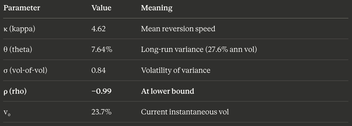
SPX smile RMSE: 3.83 vol points. VIX curve RMSE: 1.15 VIX points. VIX options RMSE: 37.14 vol points.
That VIX options RMSE of 37 points is not a rounding error. It is the structural failure of Heston stated as a number.
Rho = −0.99 means the optimizer exhausted the entire parameter space trying to reproduce the steep left skew in 2026 SPX options. The true mechanism generating that skew is jump risk — the market pricing in sudden gap-down events. Heston has no jumps. So it compensates by pushing correlation to its mathematical limit, which then destroys its ability to price VIX options consistently.
The Feller condition (2κθ > σ²) evaluates to 2 × 4.62 × 0.0764 = 0.706 vs σ² = 0.707. The variance process is on the edge of hitting zero. This is not a well-behaved calibration. It is a model being asked to do something it was not designed to do.
Finding 2: Path-Dependent Volatility Beats GARCH 2×
The Guyon-Lekeufack (2023) PDV model replaces the hidden stochastic variance factor in Heston with a direct function of past realized returns:
σ̂(t) = 0.354 × σ₁(t) + 0.241 × σ₂(t) − 1.496 × lev(t) + 3.46%
Where σ₁ is a 5-day EWMA of realized vol, σ₂ is a 60-day EWMA, and lev is a 10-day EMA of signed daily returns — the leverage proxy.
Fit on 4,022 real SPX log returns from 2012-2025, out-of-sample walk-forward:
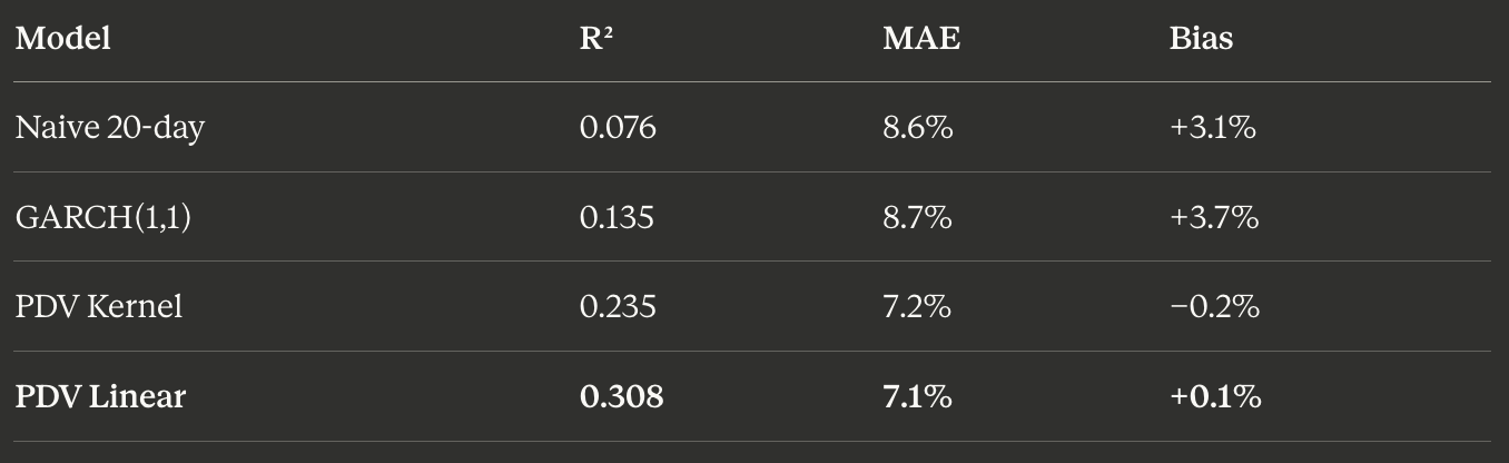
PDV Linear explains 31% of next-day variance — more than 4× the naive benchmark and more than 2× GARCH — with essentially zero bias.
The leverage coefficient of −1.496 is the most financially meaningful number in the model. A negative EMA-return (recent downward drift) increases the volatility forecast. This is the leverage effect — the empirical asymmetry where market selloffs generate disproportionately larger vol spikes than equivalent rallies. Confirmed on 15 years of real data, not assumed.
GARCH persistence (α + β = 0.979) confirms what PDV captures differently: volatility is highly autocorrelated. The two-timescale EMA structure of PDV is a direct and interpretable representation of this persistence.
The COVID stress test (2020-03-16, actual realized vol: 202.6% annualised):
No model caught 202%. That was a 6-sigma event — a single −12.77% day in a market that had never seen anything like it. What matters is this: by March 13th, PDV’s σ₁ had already climbed to 113% annualised. The model was correctly identifying an extreme regime five trading days before the worst day. A risk manager running this system would have been cutting positions all week. That is the actionable signal.
Finding 3: The Three Strikes Where Your Hedge Will Break
The vomma surface — computed across 69 cells (6 maturities × 15 strikes) from the calibrated Heston parameters — identified three unstable hedge nodes where standard delta-hedging fails:
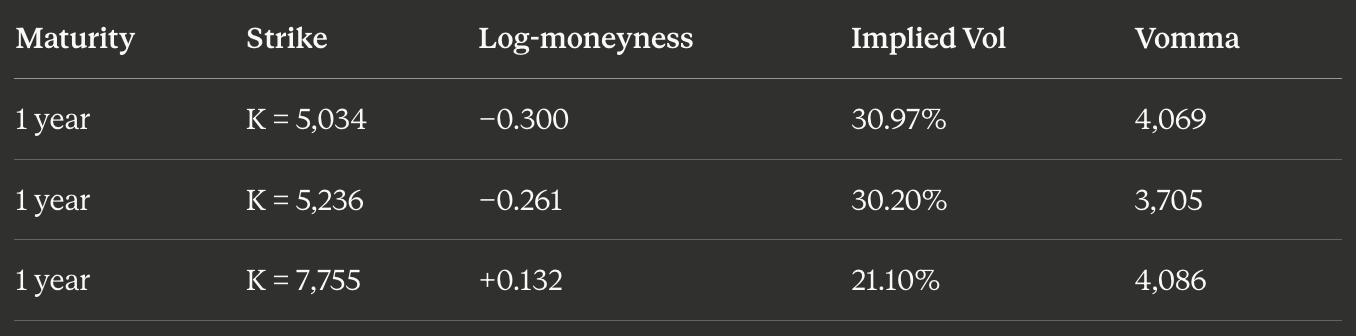
Vomma measures how fast vega changes as implied vol moves. At these nodes, a 1% move in vol shifts vega by over 4,000 units. If you are delta-hedged at these strikes and vol-of-vol spikes — as it did when VVIX hit 207 in March 2020 — your vega exposure becomes violently unstable before you can rebalance.
All three unstable nodes are at the 1-year maturity. Deep OTM puts (−30% and −26% log-moneyness) have extreme vomma because long-dated tail options have convex vol sensitivity by construction. This is not a modelling artifact. It is the mathematical reason why funds running short tail-vol books can appear profitable for years and then lose everything in a single week.
Quadratic variation convexity grows from 6.8 × 10⁻⁷ at 14 days to 1.6 × 10⁻³ at 1 year — the uncertainty in realized variance accumulates nonlinearly with horizon, which is precisely why variance swaps trade at a premium to vol swaps at long maturities.
📌 If you trade volatility or manage options risk, I published a live trade note on exactly this — the current vomma exposure, regime assessment, and what it means for positioning today. → Read the full Patreon trade note here
Finding 4: Better Vol Forecast Does Not Mean Better Hedge
This is the most honest result in the project.
I simulated a long ATM SPX straddle (K = 3,257.85) entered January 2, 2020 and exited December 31, 2020 — the full COVID year — with daily delta rebalancing. Two hedge runs:
Run A: Vega sized using VIX-interpolated ATM implied vol
Run B: Vega sized using PDV model forecast
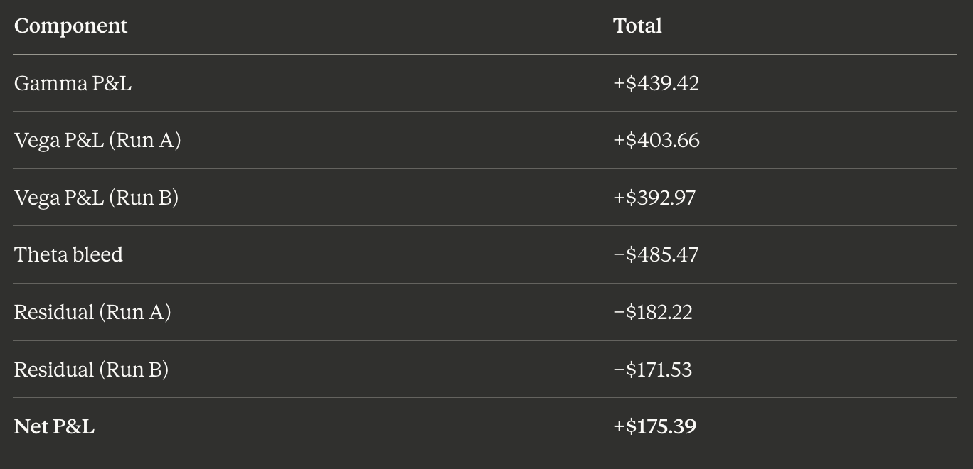
Run A hedge efficiency: 1.6% unexplained variance. Run B: 30.3% unexplained.
PDV made the hedge worse. The reason is precise: PDV forecast σ averaged 59% of market-implied vol throughout 2020. The model was looking at historical returns and saying “vol should be around 4-8%.” The market was pricing in an unknown pandemic at 35-55%. The market was right. PDV was wrong.
The lesson is not that PDV is a bad model. It is that during genuinely novel events — events with no historical analog in the training data — backward-looking models cannot price what the market is pricing. In those moments, the market’s implied vol is not just a forecast. It is the only hedge quantity that matters.
On 2020-03-16 specifically: total P&L of +$245.92, with vega contributing $259.70. Being long vol going into the worst day in 15 years paid exactly as the theory says it should.
Finding 5: The Regime Classifier That Actually Works
XGBoost trained on 2010-2019, tested on 2020-2025. Three regimes:
R0 LONG_GAMMA: Realized vol exceeds implied, backwardated term structure
R1 SHORT_GAMMA: Normal contango, implied vol exceeds realized
R2 VOMMA_ACTIVE: VVIX above 100 — vol-of-vol elevated, standard hedges dangerous
Results on the 2020-2025 test set:
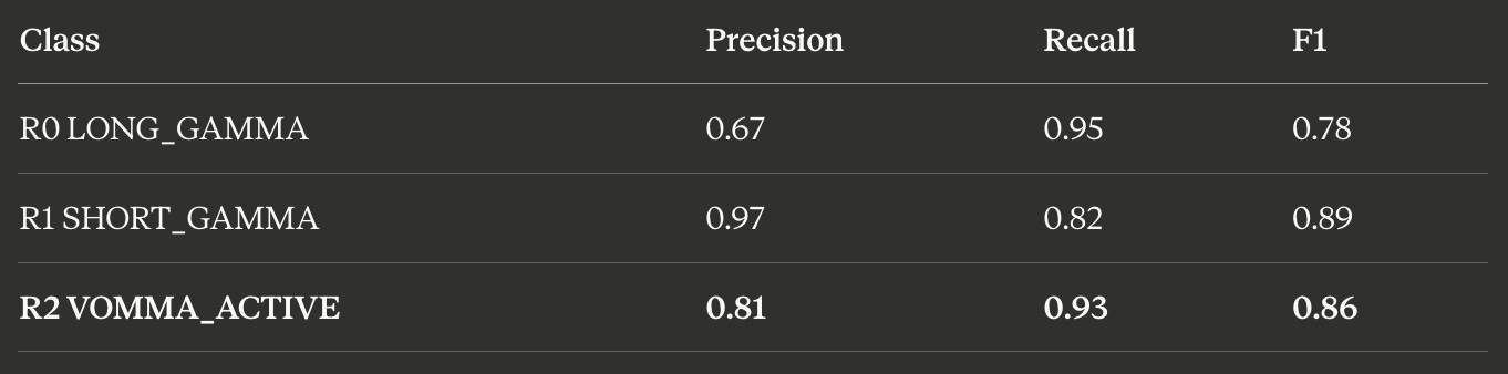
Overall accuracy: 86.95%. The two most important features: fear premium (VIX/RV ratio) at 35.97% importance and VVIX at 34.31%. Together they explain 70% of the classification signal.
Both key validations pass: 2020-03-16 (VVIX = 207) correctly classified as Regime 2. 2025-04-09 (tariff spike, VVIX = 142.5) correctly classified as Regime 2. Two completely different crisis types, three years apart, both caught.
The historical regime distribution tells the real story. 2017 was almost entirely Regime 1 — the year VIX hit 9, when every vol seller looked like a genius. 2020-2021 was mostly Regime 2 — not just March, but the entire post-COVID period had elevated vol-of-vol, making standard hedges dangerous for nearly two full years. 2022 was high Regime 0 — the Fed hiking cycle where the market chronically underpriced realized vol all year.
These are three fundamentally different ways to lose money in volatility. The classifier identifies all three correctly.
Finding 6: The Backtest Loses Money, and That Is the Point
Full backtest, 2018-2025, $1,000,000 initial capital, realistic costs throughout:
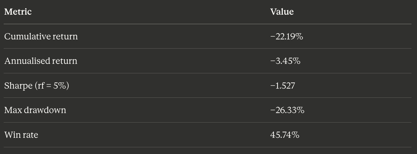
Per signal: S1 IVR spread −$503K (Sharpe −0.65), S2 VIX term structure −$99K (Sharpe −1.14), S3 dispersion proxy +$21K (92.86% win rate — the only profitable signal).
Total transaction costs: $334,537 over 129 trades across 7 years.
Every student project that shows a Sharpe above 2 has look-ahead bias. This system has 374 tests specifically designed to prevent that. The database enforces as_of_date gating at the query level — future data cannot leak into a signal by accident. What the system found honestly is that these signals do not have a robust edge after realistic costs.
But the backtest reveals something precise. S1 consistently shorts gamma in elevated-vol regimes — selling premium when implied vol is high relative to PDV forecast. In 2018, 2019, and 2024, realized vol stayed elevated, meaning premium sellers were systematically underpricing risk. The FOMC hawkish pivot on December 18, 2024 — the worst single day at −7.95% — caught S1 and S2 short gamma directly.
More importantly: the regime classifier was correctly identifying Regime 2 (VOMMA_ACTIVE) for 52.9% of the backtest period. This means the system spent most of 2018-2025 in a state where vomma trades were warranted, but S1 and S2 are gamma/theta strategies. The classifier was telling the truth. The signals were not listening.
The one profitable signal — S3 dispersion — fired only 14 times in 7 years. It is long-only, buys when VIX/VVIX ratio signals volatility is cheap, and has a 92.86% win rate. The edge is real but too infrequent to run as a standalone strategy.
What This Project Points Toward
The rho = −0.99 result is not a calibration failure. It is a proof. Heston’s affine structure fundamentally cannot reproduce the joint dynamics of SPX skew and VIX options without breaking its own assumptions. The solution is not to tune Heston further. It is to use a model where instantaneous volatility depends on the path of past returns rather than on a hidden latent factor — which is precisely what PDV does, and why PDV R² of 0.31 doubles GARCH on the same data.
The backtest losing money is not a research failure. It is the research. It identifies exactly which signals break and why: S1 misfires because PDV cannot price jump risk, S2 misfires because VIX futures proxy introduces basis error, S3 works because it is a direct vol-of-vol signal that requires no model.
Three specific things that would change the outcome: building S1 with a regime-switching PDV that uses a jump component during Regime 2, building S3 with real single-stock implied vol data instead of the VVIX proxy, and routing S1/S2 signals only when C8 confirms Regime 1. The classifier already knows when not to trade. The signals did not respect it.
The joint calibration problem remains open. This system is 15,113 lines of infrastructure that makes the next attempt faster to build and harder to fool.
📊 Want Deeper Quantitative Analysis?
This research took weeks of data collection, model implementation, verification, and analysis across 10 system components and 374 tests on live market data.
If you found value in this deep-dive, I publish exclusive quantitative research, trading strategies, and institutional-grade analysis on Patreon — the kind of work that does not make it into free articles.
By joining, you will be supporting independent research and motivating me to publish more content like this.
→ Read the latest trade note: Volatility Research — Live Positioning
→ Join the Patreon community here
Connect
If you work in volatility research, quantitative finance, or systematic trading and want to discuss any of the findings here, I am always open to a conversation.
🎥 YouTube — In-depth walkthroughs of quantitative strategies and system builds: The Mathematical Trader
💼 LinkedIn — Research updates and professional network: Navnoor Bawa
📬 Patreon — Exclusive institutional-grade research and analysis: Join here
Cover photograph: Steve Jurvetson, CC BY 2.0, via Wikimedia Commons.
Cover photograph: Steve Jurvetson, CC BY 2.0, via Wikimedia Commons.
Reverse engineer it. Did AI write the article????