


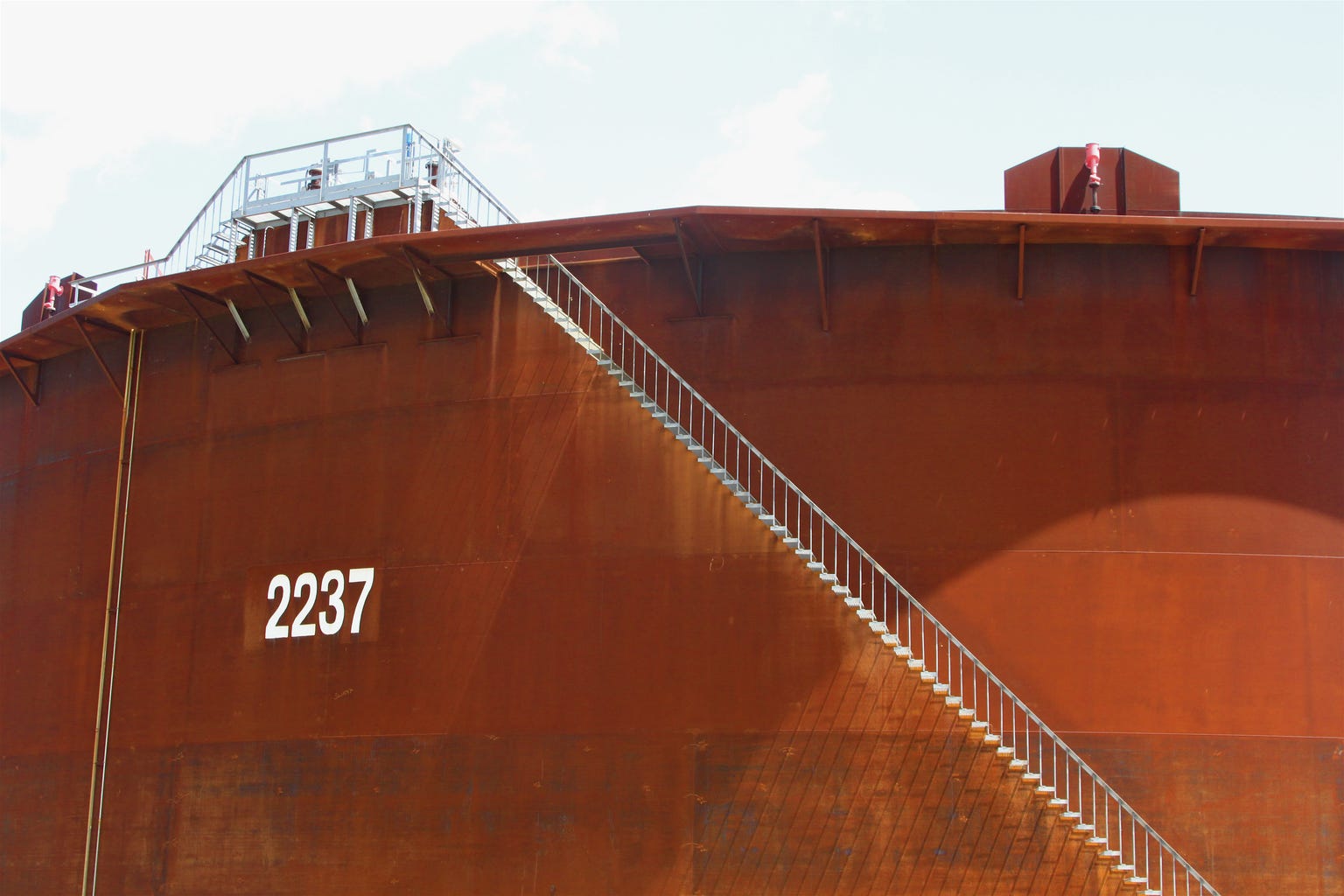
The Trade That Filled the Seas
In January 2009, as global financial markets remained in freefall, an unusual fleet began forming in ports worldwide. Not warships or cargo vessels, but oil tankers — 145 of them, to be exact — sitting idle with their cargo holds full. These weren’t transport vessels caught in a shipping slowdown. They were floating warehouses, part of what would become one of the largest commodity arbitrage trades in history.
The opportunity was unprecedented: oil for immediate delivery (spot price) traded at $40 per barrel, while contracts for delivery twelve months later fetched $60 — a $20 spread that essentially screamed “free money” to anyone with storage capacity and capital. Wall Street heard that scream loud and clear.
Goldman Sachs, Morgan Stanley, Citigroup, BP, and Royal Dutch Shell chartered massive crude carriers, creating a 30-mile convoy if placed end-to-end. They were storing approximately 100–130 million barrels of oil — enough to supply the European Union for more than three days. This wasn’t speculation on oil prices rising. This was cost-of-carry arbitrage: a textbook financial model deployed at industrial scale to lock in guaranteed profits.
The phenomenon had a name: super contango.
Cost-of-Carry 101: The Foundation
Before diving into how billions were made (and later lost), we need to understand the theoretical framework that made this trade possible.
The cost-of-carry model is fundamental to commodity derivatives pricing. At its core, it answers one question: What should a futures contract be worth relative to the spot price?
The formula is elegant:
F = S × e^((r + s — c) × t)
Where:
F = Futures price
S = Spot price
r = Risk-free interest rate (financing cost)
s = Storage cost
c = Convenience yield (benefit of holding physical commodity)
t = Time to delivery
In plain English: the futures price should equal the spot price plus the cost of storing and financing the commodity, minus any benefits from holding it physically.
Two key market structures emerge from this:
Contango: Futures price > Spot price (normal when storage costs are positive)
Backwardation: Spot price > Futures price (occurs when convenience yield exceeds carry costs, signaling scarcity)
Under normal conditions, commodities with storage costs trade in contango. You pay slightly more for future delivery because someone has to store the commodity and tie up capital. The spread typically reflects storage fees, insurance, and the opportunity cost of capital.
But in late 2008, nothing was normal.
The Setup: How Markets Created a Money Machine
The Crisis Timeline:
On July 11, 2008, WTI crude oil peaked at $147.27 per barrel. By January 2009, prices had collapsed to approximately $41.71 — a 72% plunge in six months. Yet futures prices didn’t fall nearly as fast. By early 2009, December 2009 delivery contracts traded around $20 above spot prices.
Three forces converged to create super contango:
1. Demand Destruction
The global financial crisis triggered unprecedented demand collapse. The IEA’s January 2009 Oil Market Report showed global oil demand fell to 85.3 million barrels per day — a 0.5 mb/d year-on-year decline marking the first annual contraction since 1982 and 1983. This wasn’t a typical recession dip; it was economic freefall.
2. Supply Surplus
OPEC hadn’t yet implemented meaningful production cuts. Oil continued flowing while consumption evaporated. The supply-demand imbalance flooded the market.
3. Storage Scarcity
By April 2009, the Cushing, Oklahoma storage hub (the delivery point for NYMEX WTI futures) reached 77% capacity. Land-based storage was running out.
The result? The futures curve bent into an extreme upward slope. Spot crude was essentially unwanted, while future contracts maintained value on expectations of eventual recovery.
The Arbitrage: Locking in $20 Per Barrel
Here’s how the trade worked in practice:
Step 1: Buy physical oil at $40/barrel (spot market)
Step 2: Simultaneously sell futures contract at $60/barrel for December 2009 delivery
Step 3: Store the oil (land-based or floating storage)
Step 4: Deliver against the futures contract in 12 months, pocketing the spread minus costs
The Economics:
At Cushing, land-based storage costs ran approximately $0.50-$2.00 per barrel per month (roughly $6-$24/barrel/year) — expensive and nearing capacity, but the real constraint was availability, not just price.
But tanker rates had collapsed along with shipping demand. According to industry estimates, daily rates for a million-barrel capacity Very Large Crude Carrier (VLCC) had fallen to around $10,000-$12,000 per day by late 2008 and early 2009.
Quick math on floating storage:
Estimated cost: $10,000-$12,000 per day ÷ 1,000,000 barrels = $0.01-$0.012 per barrel per day
Annual storage cost: ~$3.65-$4.38 per barrel
Financing cost: Near zero (Federal Reserve had slashed rates to 0–0.25%)
Profit calculation per barrel:
Spread: $20.00
Storage (12 months): -$3.65 to -$4.38
Financing/insurance: -$0.50 to -$1.00
Net profit: ≈$14.50-$16.00 per barrel
At scale: With 100–130 million barrels stored offshore across all participants, this represented potential profits approaching or exceeding $2 billion industry-wide.
This wasn’t a bet on oil prices rising. The futures contract was already sold. The profit was locked in on day one. The only requirements were storage access and enough capital to buy the physical oil.
The Players: Who Made Billions
While exact profit figures remain proprietary, market reporting confirmed the major participants:
Investment Banks:
Goldman Sachs
Morgan Stanley
Citigroup (Citi)
JPMorgan Chase
Oil Majors:
Royal Dutch Shell
BP
Commodity Trading Houses:
Vitol
Glencore
Trafigura
These firms had three critical advantages:
Balance sheets to purchase and hold massive oil inventories
Trading infrastructure to execute simultaneous spot and futures positions
Access to storage — whether through long-term lease agreements or direct chartering capacity
The Windfall Winners: Tanker Companies
Beyond the traders themselves, tanker companies experienced unprecedented windfalls. Firms like Frontline Ltd., Nordic American Tankers, and Altera Infrastructure saw charter rates surge as storage demand exploded. One analysis noted that tanker operators became some of the “biggest winners” from the super contango market structure, with rates soaring as traders rushed to secure what little floating storage remained.
By late 2009, one in twelve of the world’s largest oil tankers was being used for storage rather than transportation — a historic anomaly driven purely by the futures curve arbitrage.
The Unwind: When the Trade Ended
Like all convergence trades, the oil storage arbitrage had a natural expiration date — literally. As futures contracts neared delivery, the spot and futures prices converged. But profits were realized gradually as spreads narrowed throughout 2009 and early 2010.
According to industry analysis, by mid-2009, the contango spread had compressed significantly. When traders finally closed positions and delivered oil against futures contracts (or rolled to later dates), they crystallized profits.
Some traders exited early as spreads narrowed, while others held to full delivery. The key insight: the profit came from the spread compression and the financing advantage, not from oil prices rising (though some benefit accrued from the eventual recovery).
According to industry reports, by late 2009, worldwide floating storage had declined to approximately 145 vessels holding roughly 127 million barrels — down from peak levels — as contango unwound and traders took profits.
The Federal Reserve’s role was crucial. Near-zero interest rates meant the cost of financing the physical oil was minimal. Had rates been 5–6% (typical pre-crisis levels), the financing cost would have eaten significantly into profits, potentially making the trade uneconomical.
Fast Forward: The 2020 Negative Oil Catastrophe
If 2008–2009 demonstrated cost-of-carry theory in action, April 2020 revealed what happens when the model breaks catastrophically.
April 20, 2020: Oil Goes Negative
On this date, West Texas Intermediate (WTI) May 2020 futures closed at -$37.63 per barrel — the first negative oil price in history. During intraday trading, prices bottomed at -$40.32 per barrel. This wasn’t a technical glitch. Oil sellers were literally paying buyers to take barrels off their hands.
What happened?
The COVID-19 pandemic triggered simultaneous supply glut and demand collapse. IHS Markit analysis revealed that second-quarter 2020 oil demand dropped by 16.4 million barrels per day compared to the prior year — more than six times the record drop during the 2008–2009 crisis. This was unprecedented demand destruction.
Meanwhile:
Global lockdowns cratered oil consumption
OPEC+ production cuts weren’t scheduled until May 1
By March 2020, Cushing working storage capacity approached 83%
Available storage was essentially leased out
The May futures contract expired April 21. Anyone still holding contracts on April 20 faced physical delivery of 1,000 barrels per contract to Cushing, Oklahoma — where storage space no longer existed at any reasonable price.
According to the CFTC’s interim staff report on the incident, the May contracts “fell from $17.73 per barrel at the beginning of the day and eventually bottomed out at -$40.32 per barrel before settling at -$37.63.”
In a brutal 21-minute window near the U.S. market close, holders of May contracts desperately tried to exit positions. With no storage available and no buyers willing to take physical delivery, prices collapsed into negative territory. The extreme contango (May-June spread hit -$58.06 per barrel) reflected the complete breakdown in the physical market.
Key difference from 2008–2009:
In the earlier super contango, storage was accessible and expensive but available. In April 2020, storage effectively didn’t exist at any price, creating what some termed “hyper-contango” — where convenience yield turns massively negative and spot holders face extreme distress.
The Dark Side: How Retail Investors Lost Billions
While sophisticated traders with storage access profited from super contango, retail investors learned a painful lesson about negative roll yield.
The USO Disaster
The United States Oil Fund (USO) is the largest oil ETF, designed to track WTI crude oil prices by holding front-month futures contracts. Since futures expire monthly, USO must continuously “roll” its positions — selling the expiring near-month contract and buying the next month out.
In contango markets, this creates systematic losses.
Here’s why: USO sells the near-month contract (trading close to spot price) and buys the next-month contract (trading at a premium due to contango). This means the fund constantly sells low and buys high with every roll.
Example from March 2016:
Between March 7–10, USO rolled from April to May contracts:
Sold April contracts averaging $37.64
Bought May contracts averaging $39.43
Loss per contract: 4.8%
Annualized: approximately 75% cost
As one analysis noted: “Since the start of the year, front-month crude oil is up 8.3%, while USO is down 4.5% — a reflection of the roll costs from contango.”
Long-term Performance:
Research on commodity ETFs from 2008–2022 showed that USO dramatically underperformed spot oil due to persistent contango. Academic studies analyzing the fund over extended periods revealed significant negative returns that diverged substantially from spot oil price movements.
The Core Issue:
Academic research analyzing six decades of data across 19 storable commodity futures markets found that “expected returns in individual commodity futures markets are near zero before expenses” and that disappointing returns were systematically driven by the structural costs of maintaining long futures positions in contango markets. Contango reflects storage economics — and long-only futures holders pay those storage costs without capturing the arbitrage.
For passive long investors in commodity ETFs during extended contango periods, the structure bleeds value relentlessly. Unless spot prices rise faster than the roll cost, returns deteriorate.
Key Takeaways: Theory Meets Reality
The 2008–2009 super contango trade and its descendants offer crucial lessons for quantitative researchers and traders:
1. Carry Is a Cost Structure, Not a Return Forecast
Contango reflects storage, financing, and convenience yield. It does not predict future spot prices will rise. The futures curve can be in steep contango while spot prices continue falling (as happened in 2008–2009 and again in 2020).
Academic research consistently shows: the slope of the futures term structure provides limited reliable signals about expected returns for individual commodity markets.
2. Profitability Requires Arbitrage Execution
Making money from cost-of-carry models requires:
Simultaneous spot and futures positions
Access to physical or financial storage
Capital to finance the physical commodity
Ability to hold to convergence
Simply being long futures in contango markets means paying the carry without earning the arbitrage profit.
3. Negative Roll Yield Destroys Passive Positions
Commodity ETFs in persistent contango systematically underperform spot prices. For long-only investors, carry costs compound over time. One energy analyst’s 2020 analysis noted: “WTI futures are currently 3–6 times normal contango levels — which typically result in losses from roll yield of about 50% per year.”
4. Watch for Regime Changes
When convenience yield exceeds storage plus financing costs, the market signals physical strain. Backwardation or negative carry often precedes price spikes as inventories become critically low.
Conversely, super contango indicates oversupply — but this can persist for extended periods if storage remains available.
5. Storage Itself Becomes a Tradable Commodity
During periods of extreme contango, storage capacity becomes the bottleneck. In 2015, CME Group began offering oil-storage futures contracts, allowing market participants to trade the right to store specific oil types.
During 2020’s crisis, tanker companies and storage operators captured windfall profits as rates surged. One industry executive noted: “The super contango and the super profit in the crude oil market is just not there at the moment” — indicating how quickly arbitrage opportunities compress once they’re identified.
Conclusion: The Model’s Elegance and Limits
The cost-of-carry model is one of finance’s most elegant frameworks. It explains how spot and futures prices should relate under equilibrium conditions, accounting for storage, financing, and the benefits of physical ownership.
The 2008–2009 super contango demonstrated the model’s power when markets deviate from equilibrium. Sophisticated participants with infrastructure and capital extracted billions by mechanically executing arbitrage between mispriced contracts.
But the model has limits:
It assumes storage availability — but in April 2020, storage capacity constraints broke the framework entirely, sending prices negative
It describes equilibrium pricing but says little about price direction
It creates systematic losses for passive long investors in contango markets who pay the carry without executing arbitrage
For quantitative researchers, the core lesson is execution matters as much as theory.
Understanding cost-of-carry models is foundational. But profits come from recognizing when to exploit deviations (super contango with accessible storage) versus when structural headwinds will erode returns (negative roll yield for passive longs).
The difference between making $2 billion and losing 50% of your capital often lies not in the sophistication of your models, but in understanding which side of the carry trade you’re actually on.
Sources and References
Primary Sources:
CFTC Interim Staff Report: “Trading in NYMEX WTI Crude Oil Futures Contract Leading up to, on, and around April 20, 2020” (November 2020)
International Energy Agency (IEA): Oil Market Report, January 2009
U.S. Energy Information Administration (EIA): Petroleum & Other Liquids Historical Data
Commodity Futures Trading Commission (CFTC): Press Release 8315–20, Commissioner Berkovitz Statement (May 7, 2020)
Academic Research: 5. Fernandez-Perez, A., Fuertes, A., & Miffre, J. (2023). “The Negative Pricing of the May 2020 WTI Contract.” Energy Journal, 44(1), 119–142. 6. Irwin, S., Sanders, D., & Smith, A. (2018). “What Went Wrong? The Puzzle of Disappointing Commodity ETF Returns.”
Industry Analysis: 7. IHS Markit: Global Market Analysis and Commentary (2009, 2020) 8. Bloomberg Markets: “World Oil Output May Fall by 10 Million Barrels a Day, IHS Says” (March 31, 2020) 9. S&P Global Market Intelligence: IHS Markit Daily Global Market Summary (April 2, 2020) 10. Reuters Energy: Floating storage reports and market data 11. Frontline Ltd., Nordic American Tankers, and other tanker company public filings
Market Data: 12. CME Group: WTI Crude Oil Futures historical data and educational materials 13. ICE Futures: Brent Crude historical term structures 14. U.S. EIA: Cushing, Oklahoma storage capacity and utilization data
Secondary Sources: 15. “Oil-storage trade,” Wikipedia (accessed October 2025) 16. “The Great Oil Contango of 2008–2009 & Maritime Security,” Center for International Maritime Security 17. OilPrice.com: “Unprecedented Demand Destruction Marks The Return Of The Super Contango” (April 2020) 18. Wall Street Journal, Financial Times, and other financial press reports (2008–2020)
About This Series:
This article is part of an ongoing series exploring how quantitative finance concepts translate into real-world profits and losses. Each piece examines actual trades executed by hedge funds and institutional investors, with focus on understanding the mechanics behind P&L generation.
For deep dives into quantitative trading strategies that made (and lost) billions, follow this series.
Cover photograph: roy.luck, CC BY 2.0, via Wikimedia Commons.