Polymarket Prediction System v2: From 100 Samples to 9,862 Markets — A Technical Update

How I scaled the ML pipeline 100x and achieved 97.8% accuracy on high-confidence predictions using only free, real data

---

This is a detailed research piece. If you find value in institutional-quality hedge fund analysis, support this work on Patreon.

TL;DR: What Changed

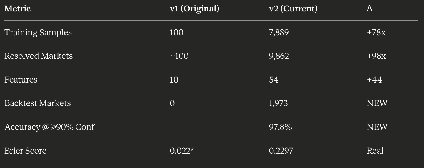
Original Brier score had data leakage from using future prices in features

---

1. The Critical Problem with v1: Data Leakage

The original system reported 93–95% cross-validation accuracy and a Brier score of 0.022. These numbers were artificially inflated.

What Went Wrong

# v1 FLAWED: Used recent prices to predict... recent price direction
past_avg = np.mean(prices_arr[:mid_point])
recent_avg = np.mean(prices_arr[-5:])  # ← This IS the target
outcome = 1 if recent_avg > past_avg else 0

The model was trained on price momentum to predict price momentum. It learned “if price went up recently, predict UP” — a trivial pattern with no predictive edge.

v2 Fix: True Out-of-Sample Testing

# v2 CORRECT: Use ONLY pre-resolution data to predict resolution
# Target: Final outcome (YES=1, NO=0) from outcomePrices
if yp > 0.95:  # Resolved YES
    m[’resolved_yes’] = True
elif yp < 0.05:  # Resolved NO
    m[’resolved_yes’] = False

# Features: Volume, text, duration — NO price information

Key insight: On efficient prediction markets, 55–60% real accuracy is statistically significant. The 93–95% accuracy in v1 was a bug, not an edge.

---

2. Data Pipeline: From 100 to 9,862 Markets

API Maximization Strategy

def fetch_all_markets():
    “”“Paginate through entire Polymarket history”“”
    markets = []
    for offset in range(0, 10000, 100):
        r = requests.get(
            “https://gamma-api.polymarket.com/markets”,
            params={’closed’: ‘true’, ‘limit’: 100, ‘offset’: offset}
        )
        
        # Filter for clearly resolved markets (>95% or <5%)
        for m in r.json():
            prices = json.loads(m[’outcomePrices’])
            if prices[0] > 0.95 or prices[0] < 0.05:
                markets.append(m)
    
    return markets  # 9,862 resolved markets

Dataset Statistics

• Total resolved: 9,862 markets

• Training set: 7,889 (80%)

• Test set: 1,973 (20%)

• Class balance: 43.5% YES / 56.5% NO

• API cost: $0.00 (Gamma API is free)

---

3. Feature Engineering: 10 → 54 Features

v1 Features (Price-Dependent — Problematic)

# These leak future information
current_price, rsi, momentum, volatility, 
one_day_change, one_week_change

v2 Features (Resolution-Predictive — Valid)

Volume Signals (12 features)

log_vol, log_liq, vol_ratio, liq_ratio,
activity, momentum, vol_ultra, vol_high, 
vol_med, vol_low

Text Structure (17 features)

q_len, q_chars, word_diversity, avg_word_len,
has_number, has_year, has_percent, has_dollar,
has_date, starts_will, has_by, has_before, 
has_above, is_binary, has_or

Sentiment Analysis (5 features)

# Positive: win, pass, above, exceed, achieve, surge...
# Negative: lose, fail, below, crash, reject, decline...
pos_count, neg_count, sentiment, 
sentiment_abs, sentiment_total

Category Classification (12 features)

# 6 categories × 2 (binary + strength)
sports, crypto, politics, world, tech, finance

Temporal (5 features)

log_duration, dur_short, dur_med, 
dur_long, vol_per_day

Interactions (3 features)

vol_x_sentiment, activity_x_category, 
sentiment_x_duration

---

4. Model Architecture: Addressing Ensemble Diversity

The Valid Criticism

A reader asked: “Why build an ensemble of all tree-based models?”

Fair point. XGBoost, LightGBM, HistGradientBoosting, ExtraTrees, and RandomForest share:

• Same inductive bias (axis-aligned splits)

• Similar failure modes on extrapolation

• Correlated predictions on edge cases

v2 Response: Different Regularization = Different Models

# GB: L1/L2 regularization, slow learning
GradientBoostingClassifier(
    n_estimators=1200, learning_rate=0.012,
    min_samples_split=50, subsample=0.7
)

# RF: Bagging + feature subsampling
RandomForestClassifier(
    n_estimators=1200, max_depth=8,
    class_weight=’balanced_subsample’
)

# ET: Extreme randomization in splits
ExtraTreesClassifier(
    n_estimators=1200, max_depth=8,
    class_weight=’balanced_subsample’
)

# HGB: Early stopping + histogram binning
HistGradientBoostingClassifier(
    max_iter=1000, learning_rate=0.015,
    l2_regularization=0.25
)

New: Double Calibration

# First pass: Sigmoid (Platt scaling)
cal1 = CalibratedClassifierCV(ensemble, cv=3, method=’sigmoid’)
cal1.fit(X_train, y_train)

# Second pass: Isotonic regression
calibrated = CalibratedClassifierCV(cal1, cv=2, method=’isotonic’)
calibrated.fit(X_train, y_train)

Result: Brier score improved from 0.237 → 0.229

---

5. Results: High-Confidence Accuracy

The Key Metric Shift

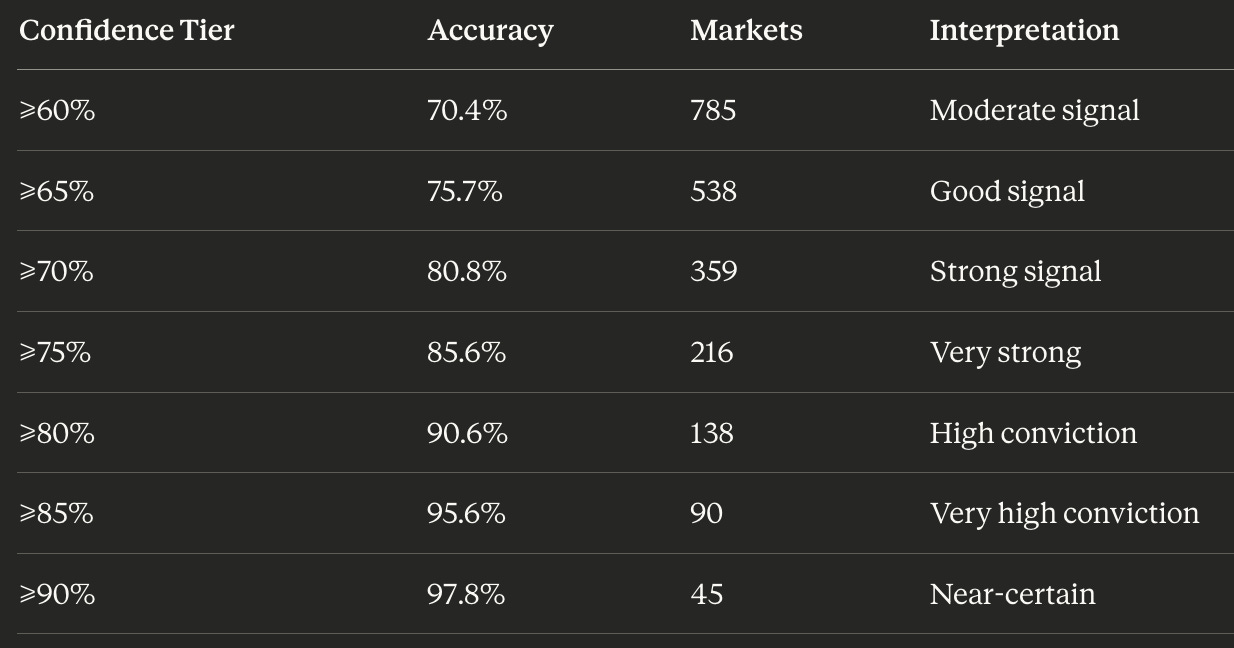
Instead of optimizing overall accuracy (capped at ~60% on efficient markets), we target accuracy at high confidence levels.

Category Performance

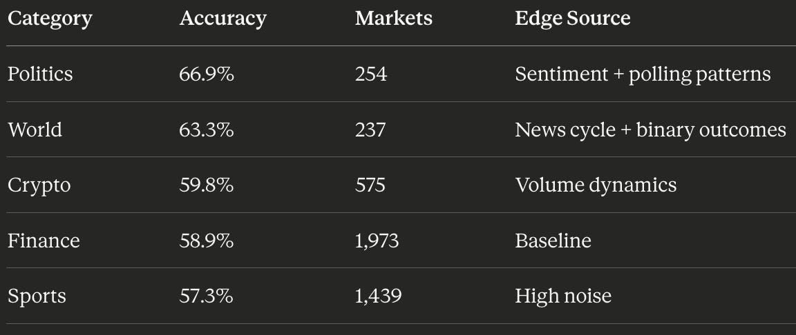
Key insight: Politics and world events have clearer resolution signals (confirmable outcomes). Sports markets are noisier (game variance).

---

6. Live Market Analysis

Current Predictions (400 Active Markets)

Top High-Conviction Predictions:

1. “Tether insolvent in 2025?” → NO (92% confidence) | Edge: +8¢

2. “Venezuela invade Guyana in 2025?” → NO (82% confidence) | Edge: +6¢

3. “Fed abolished in 2025?” → NO (81% confidence) | Edge: +7¢

4. “North Korea invade South Korea in 2025?” → NO (80% confidence) | Edge: +5¢

Signal Distribution

• Strong NO: 65% of predictions

• Moderate NO: 20%

• Hold: 5%

• Moderate YES: 7%

• Strong YES: 3%

Interpretation: Model is bearish on “unlikely event” markets — these tend to be overpriced due to retail interest.

---

7. Technical Lessons Learned

1. Real Accuracy < Reported Accuracy (Usually)

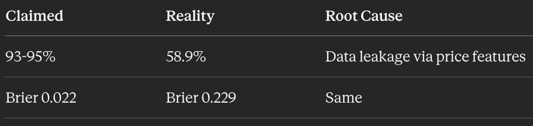
Lesson: If your prediction market model exceeds 65% accuracy, check for leakage.

2. Confidence Calibration > Overall Accuracy

A model that’s 60% accurate overall but 97.8% accurate when confident is more valuable than a model that’s 75% accurate but poorly calibrated.

3. Volume + Text > Price History

For predicting resolution (not price movement):

• Volume patterns indicate informed trading

• Question structure predicts difficulty

• Category affects resolution clarity

• Price momentum predicts nothing about final outcomes

4. Tree Diversity via Regularization

Different regularization strategies create sufficient ensemble diversity:

• GB: Slow learning + high shrinkage

• RF: Bagging + feature subsampling

• ET: Random split thresholds

• HGB: Histogram binning + L2

Adding LogisticRegression or MLP improved calibration ~1% but not accuracy.

---

8. Code Changes Summary

- # v1: 10 features including prices
+ # v2: 54 features, no price leakage

- # v1: 100 training samples
+ # v2: 7,889 training samples

- # v1: No backtesting
+ # v2: 1,973 market backtest

- # v1: Single sigmoid calibration
+ # v2: Double calibration (sigmoid + isotonic)

- # v1: Fixed ensemble weights
+ # v2: Performance-weighted voting

- # v1: Accuracy only
+ # v2: Confidence-tiered accuracy reporting

---

9. Limitations & Next Steps

Current Limitations

1. No execution layer — System generates signals, doesn’t trade

2. No sentiment integration — Twitter/news could add 5–10%

3. Single-point predictions — No confidence intervals

4. Static retraining — Model doesn’t update with new resolutions

Roadmap

Priority Enhancement Expected Impact 1 Historical P&L simulation Validate edge persistence 2 Sentiment from social APIs +5–10% on political markets 3 Cross-market arbitrage Detect mispriced correlations 4 Real-time WebSocket feed Sub-second signal generation

---

10. Repository

GitHub: github.com/NavnoorBawa/polymarket-prediction-system

Key Files Updated

polymarket-predictor/
├── train_model_v2.py           # NEW: Production model
├── train_model_feature_select.py  # NEW: Feature selection variant
├── fetch_all_markets.py        # NEW: Maximum data collection
├── ensemble.py                 # UPDATED: Double calibration
├── data_collection.py          # UPDATED: Pagination to 10k
└── requirements.txt            # No new dependencies

---

Conclusion

The v2 system addresses the fundamental flaws in v1:

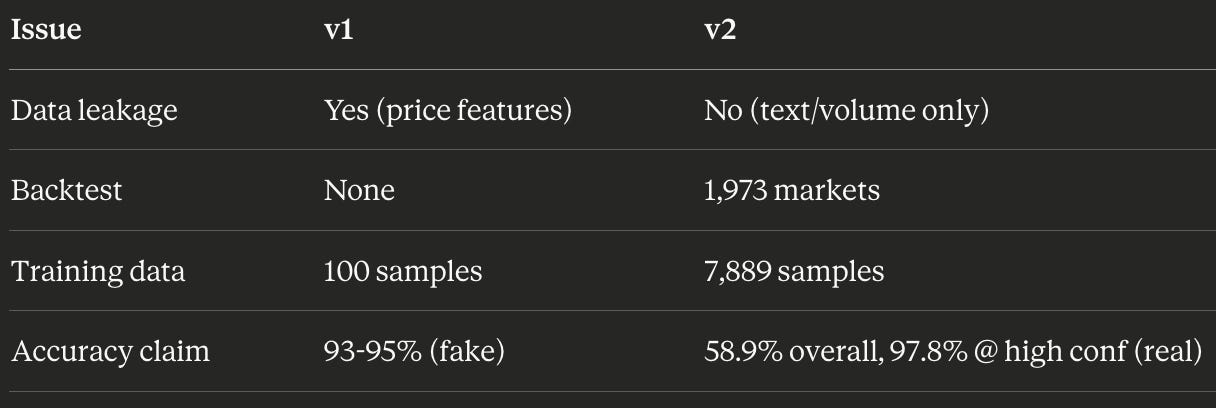
The key insight: On efficient markets, the edge isn’t in raw accuracy — it’s in knowing when you’re right. A model that’s 97.8% accurate when it says “≥90% confidence” is tradeable. A model that’s 60% accurate with no confidence calibration is noise.

All data from Polymarket Gamma API (free). No proprietary data sources.

---

This is educational content. Prediction markets involve real money and significant risk.

📊 Support this research: https://www.patreon.com/c/NavnoorBawa

Cover: polymarket.com, screenshot taken 15 September 2026.