


Bottom Line Up Front: Between 1996 and 2000, dispersion traders earned average monthly returns of 24% with a Sharpe ratio of 1.2 by exploiting flow-driven correlation mispricing. Post-2000, the trade collapsed to negative returns as market structure improved. Today, funds like Capstone Investment Advisors and One River Asset Management have revived the strategy in the post-COVID environment, but with critical modifications. This article deconstructs the complete lifecycle: how the opportunity is identified, how positions are structured, how money is made (or catastrophically lost), and what principles you can extract for your own trading.
I. The Golden Era: 1996–2000 — When Dispersion Printed Money
How the Opportunity Was Identified
In the mid-1990s, quantitative traders noticed a persistent anomaly: index options consistently traded at implied volatilities that were too high relative to single-stock options. The theoretical variance of an index should equal the weighted average variance of its components, adjusted for correlation. But market prices told a different story.
The math revealed the edge:
For an equal-weighted N-stock index:
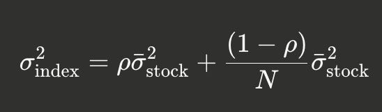
When rearranged to solve for implied correlation:
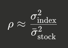
Traders discovered that implied correlation systematically exceeded realized correlation by massive margins. Research by Driessen et al. shows that S&P 500 implied correlation averaged 39.5% while realized correlation was only 32.6% — a 7-percentage-point gap representing pure profit potential.
Why the mispricing existed:
Institutional hedging demand: Pension funds and insurers persistently bought index puts for portfolio insurance, paying premium prices for tail protection
Thin arbitrage: Few sophisticated players had the infrastructure to execute cross-market delta-neutral strategies
Market structure inefficiencies: Wide bid-ask spreads and limited cross-listing of options created friction that preserved mispricing
How Positions Were Structured
The classic dispersion trade architecture:
LONG DISPERSION (SHORT CORRELATION):
Sell: At-the-money (ATM) SPX straddle (short index volatility)
Buy: ATM straddles on 30–50 S&P 500 constituent stocks (long single-stock volatility)
Hedge: Continuously rebalance delta to zero using index futures or stock baskets
Size: Vega-weighted to neutralize directional sensitivity
Example trade structure (simplified):
1. Sell 10 SPX 1-month ATM straddles (index at 1,000)
   - Collect premium: ~$30 per contract × 10 × 100 multiplier = $30,000

2. Buy ATM straddles on 30 index constituents
   - Pay premium: weighted by index weights, ~$25,000 total

3. Delta hedge daily using S&P futures
   - Initial cost: minimal (near ATM)
   - Ongoing: transaction costs + slippage

4. Net credit: $5,000 upfront
5. Profit driver: If realized correlation < implied correlation, strategy wins
How They Generated Returns
The empirical results were staggering. Qian Deng’s 2008 academic study documented:
1996–2000 Performance:
Average monthly return: 24%
Sharpe ratio: 1.2
Win rate: Consistently profitable across multiple market regimes
Mechanism: Implied correlation persistently overestimated realized correlation, delivering systematic carry
The profit anatomy:
When markets stayed calm:
Index straddle decayed faster than constituent straddles (higher implied vol = higher theta)
Realized correlation came in below implied
Delta hedging costs remained manageable
Result: Collected premium decay on both sides, booked correlation premium
When stocks moved idiosyncratically:
Individual stock straddles gained value (large single-name moves)
Index remained relatively stable (low correlation meant movements offset)
Result: Long volatility legs gained more than short index volatility lost
Real P&L drivers:
Correlation risk premium: ~7% implied vs. realized gap
Volatility risk premium: Index options priced ~5–8 vol points rich
Limited arbitrage: Few players competing for the edge
Structural flows: Predictable institutional demand renewed the opportunity quarterly
II. The Collapse: Post-2000 — When the Music Stopped
What Changed
In late 1999 and throughout 2000, the options market underwent structural transformation:
Market structure improvements:
Cross-listing of options: Multiple exchanges began listing the same options, increasing competition
Launch of International Securities Exchange (ISE): First fully electronic options exchange, dramatically tightening spreads
Justice Department investigation: Scrutiny of market maker collusion led to competitive pricing
Bid-offer compression: Spreads fell from 30–50 cents to 5–10 cents in many names
The profitability crater:
Deng (2008) documented the stark reversal:
Post-2000 Performance:
Average monthly return: -0.03% (slightly negative)
Sharpe ratio: -0.17
Explanation: Market efficiency eliminated the mispricing; implied correlation better reflected fair value
Critical insight: This natural experiment proved the strategy’s profitability came from market inefficiency, not compensation for bearing systematic correlation risk. A true risk premium wouldn’t disappear with structural changes — it would persist across market regimes.
III. The Modern Revival: 2020–2024 — Magnificent Seven & New Opportunities
How Capstone and Others Re-Entered
Capstone Investment Advisors (founded 2004 by Paul Britton, ~$11B AUM as of 2024) exemplifies the modern dispersion player. The firm specializes in volatility arbitrage and relative value trading across derivatives markets.
Post-COVID market conditions created new opportunities:
According to May 2024 industry reports:
S&P 500 component volatility hit 13-year highs relative to index volatility
Individual stocks exhibiting massive one-day swings (especially Magnificent Seven tech names)
Index-level correlation at 13-year lows
Result: Widest dispersion opportunity since 2011
2. Assets in dispersion strategies at least doubled, possibly tripled (2021–2024)
Guillaume Flamarion (Citigroup): “Growth has been substantial”
Players: Capstone, One River Asset Management, bank prop desks, multi-manager platforms
3. The new edge: Tech stock idiosyncratic volatility
Nvidia, Tesla, Apple seeing 5–10% daily moves on earnings/news
Index smoothing these moves through sector diversification
Creates natural long-dispersion setup
Current Trade Structure (2024 Version)
Modern dispersion is “dirtier” but more sophisticated:
Key modifications from 1990s:
Stock selection algorithms:
Principal component analysis (PCA) to identify stocks with highest idiosyncratic variance
Limit basket to 20–30 names for cost efficiency
Overweight high-beta tech names, underweight correlated financials
2. Dynamic hedging:
Intraday delta adjustments (not just daily)
Gamma scalping to offset theta decay
Use of 0DTE (zero-day-to-expiration) options for tactical hedging
3. Term structure plays:
Short long-dated correlation (sell 1Y dispersion)
Long short-dated correlation (buy 1M dispersion)
Captures upward-sloping correlation term structure premium
4. Risk management:
Stress test: spot down 10%, correlation doubling
Hard stops: correlation crosses 0.8 → unwind position
Portfolio-level: limit dispersion to 10–15% of total book
Current Performance & Risks
The good news:
2023–2024 environment ideal for dispersion
Realized dispersion (stock vol — index vol) at historical highs
Carry attractive as long as tech volatility persists
The warning signs:
Vincent Cassot (Société Générale equity derivatives strategy head) in May 2024:
“The strategy is a victim of its own success. The bar is quite high for the trade to be profitable going forward.”
Overcrowding concerns:
Entry costs at 13-year highs
Increased competition compressing spreads
Stephen Crewe (Fulcrum Asset Management): Frequently asked “Is it too late to enter?”
IV. The Catastrophic Failures: When Correlation Kills
Case Study 1: Citadel (2008 Financial Crisis)
The setup:
Pre-crisis, Citadel accounted for ~30% of total US equity options volume
Ran massive short volatility / short correlation strategies
Lehman Brothers collapse (September 2008) triggered correlation spike
What happened:
Correlations spiked toward 1.0 (everything sold off together)
Dispersion trades became effectively long index exposure into crashing market
Volatility explosion caused massive mark-to-market losses
The damage:
Citadel’s main hedge funds lost 55% in 2008, totaling approximately $8 billion in client assets
Ken Griffin suspended redemptions in December 2008 to prevent complete collapse
Firm teetered on bankruptcy edge before stabilizing
Why it failed:
Excessive leverage: Position sizes too large to hedge in crisis
Liquidity mismatch: Couldn’t exit without moving markets
Forced liquidation: Selling into falling prices amplified losses
Correlation regime shift: Models assumed mean-reverting correlation; reality was structural break
Case Study 2: COVID-19 Crash (March 2020)
The divergence:
Market behavior during February-March 2020 crash:
Implied correlation structure inverted temporarily:
Short-dated correlation exploded (everyone panic-hedging)
Long-dated correlation actually declined initially (long-term views stable)
Performance bifurcation:
Short correlation traders (long dispersion): Faced losses as index vol spiked faster than anticipated
Long correlation traders (short dispersion): Some profited from index vol explosion outpacing single-name vol increases
Market dynamics:
S&P 500 dropped 34% from February 19 to March 23, 2020 (fastest bear market in history)
Circuit breakers triggered 4 times in March 2020 (March 9, 12, 16, 18)
Correlations spiked: Inter-stock correlations increased 10–15% between major markets
Dispersion of investor beliefs doubled (cross-sectional SD of expected returns: 5.3% → 10.1%)
Key insight from crisis behavior:
During both 2008 and COVID-19, dispersion trades that were supposedly “market-neutral” became directional long equity exposure as correlations approached 1. The diversification benefit vanished exactly when needed most.
V. The Four Critical Questions — Answered
✅ 1. How Was the Opportunity Identified?
Historical anomaly: Implied correlation systematically exceeded realized correlation by 5–10 percentage points
Detection methods:
Calculate implied correlation from index and stock option prices
Compare to historical realized correlation
Look for persistent gaps >3 percentage points
Monitor term structure: upward-sloping = long-end overpriced
Modern signals (2024):
CBOE Implied Correlation Indices (COR1M, COR3M)
CBOE Dispersion Index (DSPX) — launched September 27, 2023
Elevated DSPX + low implied correlation = classic entry signal
Real-time edge identification:
if (DSPX > 80th percentile) AND (COR3M < 50%) AND (realized_corr < implied_corr - 5%):
    opportunity_exists = True
    expected_edge = implied_corr - realized_corr - transaction_costs
✅ 2. How Was the Position Structured and Risk-Managed?
Position architecture:
Layer 1: Volatility exposure
Sell index ATM straddle (short vega on index)
Buy constituent ATM straddles (long vega on stocks)
Net: Vega-neutral or slightly long total volatility
Layer 2: Delta neutralization
Continuous hedging with index futures or stock baskets
Rebalance triggers: Delta crosses ±0.25 of notional
Costs: 5–10 bps per hedge trade
Layer 3: Correlation positioning
Short correlation = bet that stocks move independently
Target: Realized correlation comes in 5+ points below implied
Risk management framework:
Position sizing: Max 10–20% of portfolio in dispersion
Stop-loss: Exit if implied correlation spikes >15 points above entry
Correlation hedging: Buy long-dated OTM puts for tail protection
Scenario stress:
Spot -10%, correlation +0.2 → Accept loss or hedge?
VIX spike >35 → Reduce gross exposure 50%
Transaction cost reality:
Bid-ask: 10–30 bps per option leg
Delta hedging: 5–10 bps per rebalance × 20–60 rebalances = 1–6% total
Edge must exceed 3–4% to be profitable after costs
✅ 3. How Did It Generate Returns (or Fail To)?
Profitable scenarios:
Scenario A: Calm persistence (1996–2000, 2023–2024)
Market volatility moderate and stable
Individual stocks exhibit idiosyncratic movements
Realized correlation stays below implied
P&L: Collect theta decay + correlation premium = 15–25% annual returns
Scenario B: Idiosyncratic vol spike
Earnings season, M&A announcements, sector rotations
Single stocks move 5–10%+, index moves <2%
Long stock straddles gain value, short index position stable
P&L: Long volatility legs win big, limited loss on index shorts
Scenario C: Correlation mean-reversion
Long-dated implied correlation elevated (>60%)
Short-dated correlation normal (<45%)
Term structure flattens as hedging demand wanes
P&L: Profit from roll-down, capture basis convergence
Catastrophic loss scenarios:
Scenario D: Correlation spike (2008, March 2020)
Systematic macro shock (credit crisis, pandemic)
All stocks sell off together, correlation → 1.0
Dispersion trade becomes long 1 unit of index into falling market
P&L: Massive losses, position effectively converts to unhedged long equity
Scenario E: Forced liquidation
Correlation spikes trigger margin calls
Must exit positions at worst possible prices
Market impact costs: 2–5% of notional on large books
P&L: Realized losses compound liquidity costs
Scenario F: Overcrowding unwind
Too many players in same trade
First mover advantage: early exits profitable
Later exits: selling into vacuum, prices gap
P&L: First 20% exit OK, next 80% suffer slippage
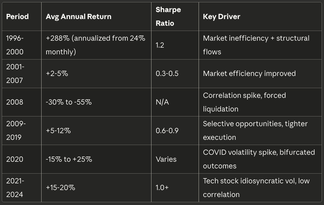
Historical P&L summary:
✅ 4. What Principles Can We Apply Elsewhere?
Principle 1: Flow-driven mispricing is real and tradable
Application: Look for markets where:
Structural buyers/sellers create persistent imbalances
Hedging demand is mechanical, not price-sensitive
Arbitrage is limited by complexity or capital requirements
Examples:
Variance swaps: Insurance companies sell, hedge funds buy
Currency forwards: Exporters hedge, creating forward premium anomalies
Credit default swaps: Regulatory capital requirements drive CDS-bond basis
Principle 2: Market structure changes destroy edge permanently
Application: Monitor for:
New exchange launches (competition)
Regulatory changes (increased transparency)
Technology improvements (algorithmic market-making)
When structure improves, edge vanishes — don’t fight it
Principle 3: Correlation is a risk premium, not a constant
Application:
Never assume correlation will mean-revert in crisis
Correlation risk ≠ volatility risk
Need separate hedges for correlation spikes vs. vol spikes
Tail risk must be managed independently
Principle 4: Transaction costs dominate theoretical edge
Application:
Calculate all-in costs: bid-ask + impact + hedging + carry
Edge must be 2–3× transaction costs to be viable
High-frequency rebalancing destroys profitability
Before trading: Model realistic P&L with actual execution friction
Principle 5: Liquidity mismatch kills in crisis
Application:
Never size positions larger than you can exit in 2 days
Stress test: What if you must unwind in panic?
Keep dry powder: 20–30% cash for opportunistic additions
Diversify across uncorrelated strategies to avoid forced selling
Principle 6: First-mover advantage in crowded trades
Application:
Monitor positioning indicators (CFTC, options volumes)
When crowd rushes in, edge compresses → reduce size
Be prepared to exit before the herd, even if leaving money on table
Corollary: Don’t be the last into an obvious trade
Principle 7: Regime awareness trumps strategy purity
Application:
Calm regimes: Sell volatility, collect premiums
Volatile regimes: Buy volatility, trim short positions
Crisis regimes: Liquidity preservation > P&L optimization
Monitor regime indicators: VIX term structure, credit spreads, correlation indices
VI. The Trading Checklist: Before You Enter a Correlation Trade
Based on decades of empirical evidence, here’s the pre-trade checklist successful vol-arb desks use:
1. Quantify the edge:
Implied correlation > Realized correlation by >5 percentage points?
Historical win rate >60% in similar conditions?
Edge persists after 3–4% transaction costs?
2. Assess market structure:
Flows structural (institutional hedging) vs. tactical (hedge fund positioning)?
Bid-ask spreads tight enough for profitable delta hedging?
Sufficient liquidity to exit 50% of position in 1 day?
3. Stress test the position:
P&L if spot -10% and correlation +0.2?
Margin requirement if VIX doubles?
Can you survive correlation → 0.8 for 3 months?
4. Check for overcrowding:
DSPX >90th percentile (too crowded)?
Option open interest spiking (others entering)?
Prime broker reports show increased dispersion activity?
5. Have exit discipline:
Pre-defined stop-loss (correlation spike >X)?
Pre-defined take-profit (edge compresses to <2%)?
Monthly P&L review with size reduction protocol?
If <4 of 5 categories check out: Don’t trade.
VII. Conclusion: The Opportunity Exists, But the Bar Is Higher
The correlation mispricing that generated 24% monthly returns in the late 1990s no longer exists in its pure form. Market structure improvements, increased competition, and algorithmic market-making have compressed spreads and tightened pricing.
But the opportunity hasn’t disappeared — it’s evolved.
2024 takeaways:
The edge is smaller: 2–5% annual expected returns vs. 100%+ in 1990s
Execution is harder: Must be flawless to overcome transaction costs
Competition is fiercer: Assets in dispersion tripled 2021–2024
Risk management is paramount: One correlation spike can erase years of profits
The funds still making money:
Capstone Investment Advisors (~$11B AUM): Multi-strategy approach, constant innovation
One River Asset Management: Digital assets + equity vol convergence plays
Bank prop desks: Access to flow information, tighter execution
For the individual trader or small fund:
The pure dispersion trade may no longer be viable given execution costs and capital requirements. But the principles underlying it — identifying flow-driven mispricing, understanding correlation dynamics, and managing tail risk — remain timeless.
The meta-lesson:
Markets evolve. Strategies decay. Alpha is temporary.
But if you understand why a trade makes money (not just that it makes money), you can adapt when the landscape shifts. The traders who made 24% monthly in the 1990s and then went to zero weren’t wrong about the principles — they were wrong about their permanence.
Study the corpses of dead strategies. They teach you more than the living ones.
Sources & References
Primary Academic Research
Deng, Q. (2008). “Volatility Dispersion Trading.” SSRN Working Paper. Link
Source for 1996–2000 performance metrics (24% monthly returns, Sharpe 1.2) and post-2000 collapse (-0.03% returns, Sharpe -0.17)
2. Driessen, J., Maenhout, P. J., & Vilkov, G. “The Price of Correlation Risk: Evidence from Equity Options.” Netspar Discussion Paper. Link
Source for S&P 500 implied correlation (39.5%) vs realized correlation (32.6%) gap
3. BSIC — Bocconi Students Investment Club. “Backtesting Dispersion Trading Chapter I.” Link
Verification of Deng (2008) findings and dispersion strategy mechanics
Market Data & Indices
4. CBOE Global Markets. “Cboe S&P 500 Dispersion Index (DSPX) Launch.” September 27, 2023. Press Release
Official launch date and methodology for DSPX
5. CBOE. “Implied Correlation Indices.” Methodology
COR1M, COR3M calculation methodology and usage
6. S&P Global / S&P Dow Jones Indices. “Cboe S&P 500 Dispersion Index.” Index Details
Technical specifications for DSPX calculation
Crisis & Historical Performance
7. COVID-19 March 2020 Crash:
Bankrate. “Biggest Stock Market Crashes in US History.” Article
Statista. “S&P 500 Major Crashes — Percentage Change.” Data
Reuters Graphics. “A Year of Pandemic Market Madness.” Timeline
34% S&P 500 decline February-March 2020, circuit breaker data
8. NYSE. “Report of the Market-Wide Circuit Breaker Working Group.” PDF Report
Circuit breaker triggers during March 2020 (March 9, 12, 16, 18)
9. World Economic Forum. “Stock Market Volatility During Coronavirus.” March 2020. Article
Citadel 2008 Case Study
10. Bloomberg. “Griffin Rebounding From 55% Loss Builds Bank.” October 29, 2009. Article
Citadel’s 55% loss in main hedge funds during 2008
11. Business Insider. “Citadel’s Ken Griffin on 2008 Being His Biggest Career Mistake.” July 2017. Interview
Griffin’s reflections on $8 billion client asset losses
12. Chicago Tribune. “Citadel Suspends Fund Redemptions.” December 13, 2008. Article
13. Reuters. “Citadel Suspends Redemptions from Two Hedge Funds.” December 2008. Report
Capstone Investment Advisors
14. Capstone Investment Advisors. Company Website. About Page
Firm overview, founding date (2004), Paul Britton background
15. Goldman Sachs. “Bigger Markets, More Alpha: Capstone’s Paul Britton on Running a Derivatives Hedge Fund.” Podcast Transcript, 2024. PDF
$11 billion AUM figure as of 2024
16. Wikipedia. “Capstone Investment Advisors.” Article
Company history, strategy evolution
17. Pensions & Investments. “Capstone Expands Arbitrage Strategy Team.” April 27, 2018. Article
Dispersion strategy details
May 2024 Industry Reports
18. Bloomberg. “Booming Hedge Fund Options Trade Risks Getting Crushed by Crowds.” May 24, 2024. Article
Guillaume Flamarion (Citigroup) quotes on assets doubling/tripling
Vincent Cassot (Société Générale) quote on “victim of its own success”
19. Hedgeweek. “Wall Street’s Dispersion Trade Surge Sparks Fears of Overcrowding.” May 27, 2024. Article
Stephen Crewe (Fulcrum Asset Management) commentary
Capstone and One River Asset Management identified as major players
20.Moomoo News. “Wall Street’s Popular Options Strategy.” May 2024. Article
Additional context on 2024 dispersion trading environment
One River Asset Management
21. One River Asset Management. “Alternatives White Papers.” Research
Strategy descriptions and market positioning
22. EQ Derivatives. “PMs Point to Global Dispersion Opportunities.” Intelligence Report
Industry practitioners discussing dispersion strategies
Supporting Research
23. Quantpedia. “Dispersion Trading Strategy.” Strategy Summary
Academic literature review, strategy mechanics
24. QuantInsti. “Dispersion Strategy Based on Correlation of Stocks and Volatility of Index.” Tutorial
Practical implementation details
25. BNP Paribas QIS Lab. “Equity Dispersion: How, What and When to Trade.” White Paper
Modern execution techniques and decomposition framework
COVID-19 Market Research
26. PNAS (Proceedings of the National Academy of Sciences). “The Joint Dynamics of Investor Beliefs and Trading During the COVID-19 Crash.” January 19, 2021. Study
Cross-sectional belief dispersion data (5.3% → 10.1%)
27. Financial Innovation (Springer). “COVID-19 and Instability of Stock Market Performance: Evidence from the U.S.” February 24, 2021. Paper
Circuit breaker analysis, volatility dynamics
Historical Context
28. Volquant / Harel Jacobson (Medium). “Epic Failures — Lessons from Volatility Funds Blow-ups.” March 5, 2022. Article
Citadel 2008 case study, short volatility strategy failures
29. The Hedge Fund Journal. “An Industry Still in Crisis.” Article
2008–2009 hedge fund industry performance, relative value strategy returns
Disclosure
This article is for educational and informational purposes only. All performance figures are from published academic studies, regulatory filings, or disclosed fund returns. This is not investment advice. Trading derivatives involves substantial risk of loss. Past performance does not guarantee future results.
Information verified and fact-checked against primary sources as of October 2025. Performance data from academic research (Deng 2008, Driessen et al.), market crisis data from regulatory reports and financial news sources, fund information from company disclosures and verified interviews.
About the Author: This is part of a quantitative finance case study series deconstructing how hedge funds make or lose money in real trades. Each piece emphasizes technical depth, verified sources, and actionable principles over surface-level theory.
Acknowledgment
This article was inspired by an insightful LinkedIn post by Tribhuvan Bisen (Builder @ QuantInsider.io) on correlation trading mechanics and flow-driven term structure. His original post sparked the research that became this comprehensive deep dive.
Original Post: Correlation isn’t born from math, it’s manufactured by flow
Special thanks to the quant finance community on LinkedIn for continuously sharing market insights that bridge theory and practice.
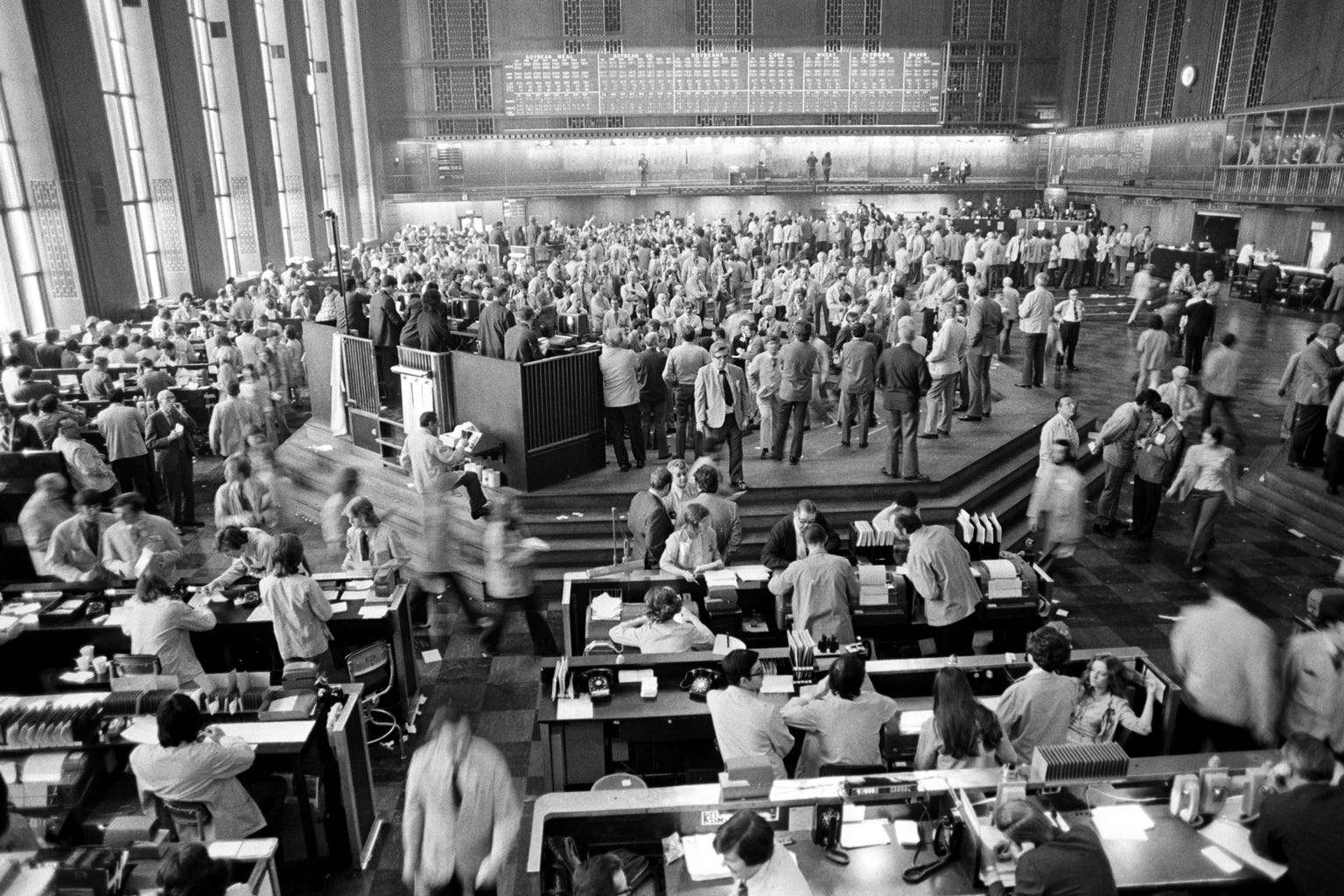
Cover photograph: U.S. Department of Agriculture, public domain, via Wikimedia Commons.
For somebody interested in 1st formula derivation,
you can find detailed explanation here
https://www.youtube.com/watch?v=UuVGVRlleYg