



August 2007. Goldman Sachs’ Global Equity Opportunities Fund lost over 30% in one week. Renaissance Technologies’ Institutional Equities Fund dropped 8.7% for the month. Highbridge Statistical Opportunities fell 18%. AQR Capital Management’s flagship fund hemorrhaged 13% in ten days.
Collective damage: Over $150 billion in mark-to-market losses across the quantitative hedge fund industry.
This wasn’t a market crash. The S&P 500 barely moved. No economic catalyst emerged. What destroyed these funds was systematic misuse of the Sharpe ratio — the metric these PhD mathematicians relied on to measure risk.
Nine years earlier, an eerily similar disaster unfolded. Long-Term Capital Management (LTCM) — co-founded by Myron Scholes and Robert Merton, 1997 Nobel Prize winners — lost $4.6 billion in four months. Leverage exceeded 250:1. The Federal Reserve orchestrated an emergency $3.6 billion bailout to prevent global meltdown.
The pattern: The world’s most sophisticated investors keep making identical statistical errors. And it keeps costing billions.
A September 2025 paper by Marcos López de Prado (Global Head of Quantitative Research, Abu Dhabi Investment Authority), Alexander Lipton, and Vincent Zoonekynd addresses this systematically. “How to Use the Sharpe Ratio” identifies five critical statistical pitfalls that explain why naive Sharpe ratio analysis leads to catastrophic decisions.
This article deconstructs exactly how the money was lost — and provides the framework to prevent it from happening again.
Part I: LTCM — The $4.6 Billion Failure of Nobel Prize Math
The Dream Team
January 1998. Long-Term Capital Management held ~$129 billion in assets with $4.7 billion in equity — leverage exceeding 27:1. Including off-balance-sheet derivatives ($1.25 trillion notional), effective leverage exceeded 250:1.
Context: For every dollar of capital, LTCM controlled over $250 of market exposure. Equivalent to buying a $1 million home with less than a $4,000 down payment.
The founders:
John Meriwether (former Salomon Brothers vice chairman)
Myron Scholes & Robert Merton (1997 Nobel laureates)
David Mullins (former Federal Reserve vice chairman)
Elite Salomon traders
Early success (1994–1997):
1994: 21% (after fees)
1995: 43%
1996: 41%
1997: 17%
By December 1997, LTCM managed ~$7 billion. Their strategy: exploit tiny pricing inefficiencies in fixed-income markets through convergence arbitrage. Using sophisticated models, they identified bonds theoretically mispriced relative to each other, betting spreads would converge.
Their models said it was virtually risk-free when properly hedged.
The Five Fatal Statistical Errors
Error #1: The Normality Assumption
LTCM calculated daily Value at Risk (VaR) of $45 million, believing their risk profile matched simply investing in the S&P 500. But this VaR deliberately excluded crisis periods (1987, 1994), assuming returns followed normal distributions during “normal” times.
In August 1998, LTCM experienced an 8.3 standard deviation event — something their models said should occur once every 6.4 trillion years.
The problem: Financial markets don’t follow normal distributions. They exhibit fat tails and negative skewness — small gains punctuated by catastrophic losses.
Error #2: Neglecting Statistical Significance
LTCM’s VaR was independent of fundamental risk factors. The models couldn’t distinguish between temporary volatility and structural risk. They were neutral on whether debt levels were high or low, spreads widening or tightening, currencies pegged or free-floating.
Error #3: Insufficient Test Power
Models tested on limited historical data that didn’t capture extreme correlation breakdowns. When Russia unexpectedly defaulted (August 17, 1998), spreads didn’t converge — they exploded.
August alone: LTCM lost 44% of value. By September 25, equity plummeted from $4.7 billion to $400 million. With liabilities exceeding $100 billion, leverage surged past 250:1.
Error #4: Multiple Testing Not Corrected
LTCM tested numerous strategies and parameters but never adjusted for the fact that finding profitable patterns after extensive testing is statistically meaningless without multiple testing corrections.
Error #5: Ignoring Sample Size Requirements
With only 36 months of track record showing Sharpe ratios around 2.0, LTCM launched with insufficient statistical evidence that their edge was real versus noise.
The Death Spiral: How $4.6 Billion Evaporated
August 17, 1998: Russia devalues ruble, declares moratorium on 281 billion rubles ($13.5 billion) of Treasury debt.
Flight to quality: Investors flood into safest government bonds. LTCM’s convergence trades move violently against them.
Mark-to-market losses: Position values deteriorate; collateral value declines.
Margin calls: Banks demand additional capital. LTCM must post more collateral or liquidate.
Forced liquidation: Selling in illiquid markets amplifies losses. Each sale pushes prices further against them.
Correlation breakdown: “Hedged” positions become 90%+ correlated. Hedges fail simultaneously.
Feedback loop: Losses → margin calls → forced selling → more losses.
System-wide threat: With $1.25 trillion in derivative exposure, LTCM’s collapse threatens global finance.
Federal Reserve Chairman Alan Greenspan: “Had the failure of LTCM triggered the seizing up of markets, substantial damage could have been inflicted on many market participants, including some not directly involved with the firm, and could have potentially impaired the economies of many nations.”
September 23, 1998: Federal Reserve Bank of New York orchestrates $3.6 billion bailout involving 14 major institutions.
Part II: August 2007 — When Everyone Ran the Same “Unique” Strategy
The Quant Meltdown
August 6–9, 2007. Quantitative long/short equity hedge funds experienced unprecedented losses concentrated among market-neutral statistical arbitrage strategies.
Verified losses:
Goldman Sachs Global Equity Opportunities: Lost over 30% in one week
Renaissance Institutional Equities Fund: Down 8.7% for August 2007 (year-to-date: -7.4%)
Highbridge Statistical Opportunities: Down 18% by August 8
AQR Capital Management flagship: Down 13% in first 10 days of August
Goldman Sachs Global Alpha: Lost 22.7% in August
What made these losses extraordinary: They occurred during relative calm. On August 7–8, when quant funds hemorrhaged billions, the S&P 500 moved less than 1%.
The Trade Architecture
By 2007, quantitative equity funds managed over $40 billion (up significantly from approximately $10 billion in 2004). Most employed variations of the same factor-based strategies:
Long positions:
Value stocks (high book-to-market, cash flow-to-price)
Quality stocks (strong balance sheets)
Positive momentum stocks
Short positions:
High-valuation growth stocks
Low-quality companies
Negative momentum stocks
Leverage: Typically 3–8x, targeting 15–40% annual returns on 2–5% underlying edges.
These strategies posted excellent backtested Sharpe ratios: typically 1.5–2.5, sometimes exceeding 3.0. On paper, they were printing money with minimal risk.
The Same Five Errors, Different Fund
Error #1 (Normality): Backtests assumed normal return distributions. Reality: fat tails and negative skewness.
Error #2 (Statistical Significance): Nobody verified whether observed Sharpe ratios were statistically significant given sample sizes and return characteristics.
Error #3 (Test Power): Insufficient out-of-sample testing and stress testing under extreme conditions.
Error #4 (Multiple Testing): Every shop tested hundreds of factors. All discovered the same ones “worked”: value, quality, momentum. But no one corrected for the fact that finding a 2.0 Sharpe ratio after testing 500 factors is meaningless without adjustment.
If you test 1,000 random noise strategies, you’d expect some to show Sharpe ratios of 2.0+ just by chance.
Error #5 (Crowding/Correlation): Everyone held identical positions. When one fund hit risk limits, everyone did simultaneously.
The Cascade: Minute by Minute
Using high-frequency data, MIT researchers Amir Khandani and Andrew Lo identified two specific unwinds:
August 1, 2007, 10:45 AM: Mini-unwind begins (lasts until 11:30 AM). Large fund with mortgage exposure begins deleveraging.
August 6, Market Open: Sustained unwind begins, starting with financials and value factors.
Mechanics:
Forced selling of longs (value stocks drop 5–8%)
Forced covering of shorts (growth stocks rally 3–5%)
Result: Exact opposite of what models predicted
The Amplification:
Day 1 (August 6): Small fund hits stop-loss → begins liquidating positions.
Day 2 (August 7): Price movements trigger stop-losses at other funds → synchronized liquidation.
Day 3 (August 8): Widespread panic. Anyone running similar strategies experiences:
Long positions down 5–10%
Short positions up 3–7%
Net: Catastrophic losses
The correlation spike: Strategies that backtested with 0.3–0.5 correlation suddenly exhibited 0.95+ correlation during the unwind.
Why? They weren’t running “different” strategies. They were running the same strategy with different labels.
The Exception That Proves The Rule: Renaissance Medallion
While most quant funds imploded, Renaissance Technologies’ Medallion Fund — closed to outside investors — posted strong positive returns in 2007 despite the August crisis.
Same market. Same crisis. Opposite result.
What was different?
Medallion’s approach:
Proprietary signals (not publicly available factors)
Extreme diversification (thousands of uncorrelated bets)
Rigorous statistical testing with multiple testing corrections
Short holding periods (reducing tail risk exposure)
Conservative leverage relative to signal quality
Renaissance’s internal Institutional Equities Fund (RIEF) — which did use common factors — lost 8.7% in August 2007. This wasn’t coincidence. It was statistical proof that common factor strategies had become overcrowded.
The contrast between Medallion and RIEF demonstrates the critical difference: Medallion avoided the five statistical errors that destroyed others.
Part III: The Statistical Solution Framework
What the Sharpe Ratio Actually Measures
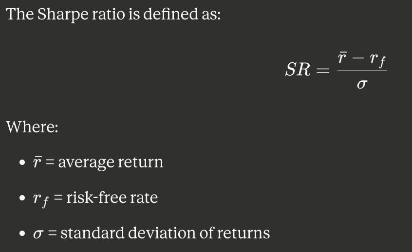
The fundamental problem: This assumes returns are normally distributed and independent. Financial returns violate both assumptions.
The Probabilistic Sharpe Ratio (PSR)
López de Prado’s framework introduces the Probabilistic Sharpe Ratio — the probability that the estimated Sharpe ratio exceeds a benchmark after accounting for:
Non-normality (skewness and kurtosis)
Sample size
Estimation uncertainty
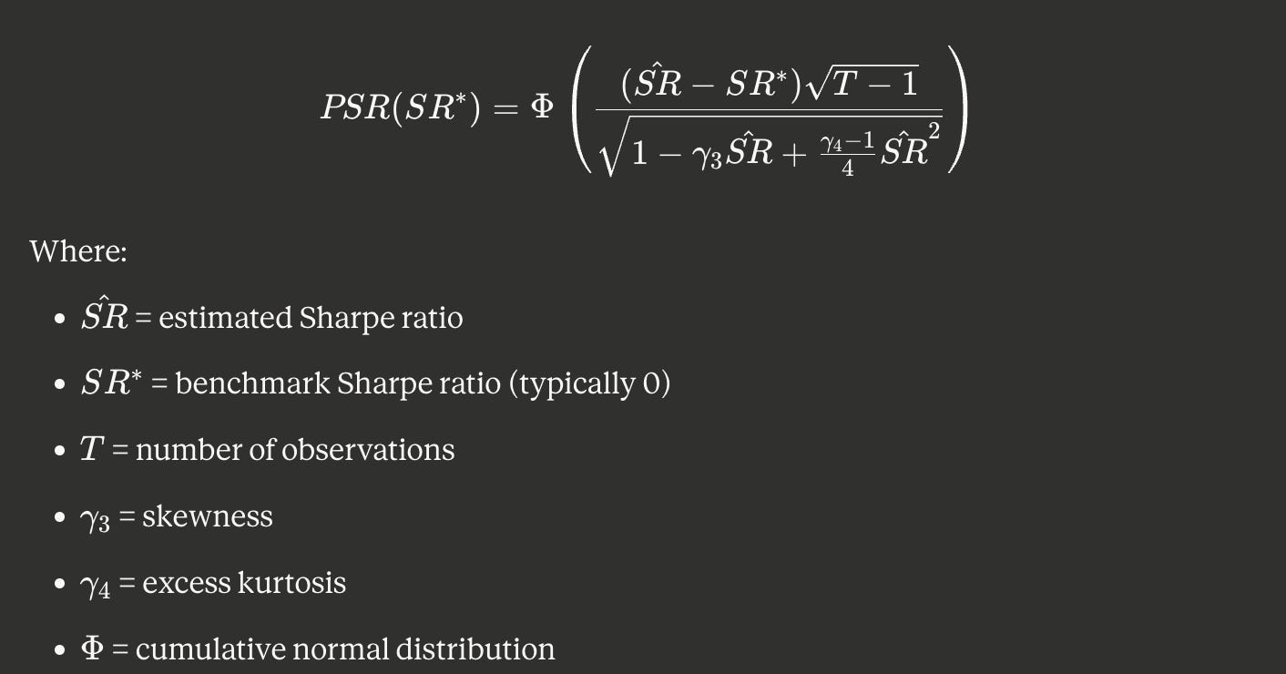
Interpretation: PSR(0) = 0.95 means 95% confidence your strategy has positive Sharpe ratio.
Python Implementation
import numpy as np
from scipy.stats import norm, skew, kurtosis

def probabilistic_sharpe_ratio(returns, benchmark_sr=0.0):
    “”“
    Calculate Probabilistic Sharpe Ratio

    Parameters:
    -----------
    returns : array-like
        Strategy returns (not cumulative)
    benchmark_sr : float
        Benchmark Sharpe ratio to test against (default 0)

    Returns:
    --------
    psr : float
        Probability that true SR exceeds benchmark_sr
    estimated_sr : float
        Estimated Sharpe ratio from sample
    “”“
    returns = np.array(returns)

    # Calculate moments
    T = len(returns)
    mean_return = np.mean(returns)
    std_return = np.std(returns, ddof=1)
    skewness = skew(returns, bias=False)
    kurt = kurtosis(returns, bias=False, fisher=True)  # Excess kurtosis

    # Estimated Sharpe ratio (assuming rf=0 for simplicity)
    estimated_sr = mean_return / std_return * np.sqrt(252)  # Annualized

    # PSR calculation
    numerator = (estimated_sr - benchmark_sr) * np.sqrt(T - 1)
    denominator = np.sqrt(1 - skewness * estimated_sr +
                         ((kurt) / 4) * estimated_sr**2)

    psr = norm.cdf(numerator / denominator)

    return psr, estimated_sr

# Example: LTCM-style strategy
np.random.seed(42)
# Simulate returns: high mean, low vol, but negative skew and fat tails
returns = np.random.standard_t(df=5, size=756) * 0.01 + 0.002  # ~3 years daily

psr, sr = probabilistic_sharpe_ratio(returns)
print(f”Estimated Sharpe Ratio: {sr:.2f}”)
print(f”Probabilistic Sharpe Ratio: {psr:.4f}”)
print(f”Confidence strategy has positive SR: {psr*100:.1f}%”)
Minimum Track Record Length (MinTRL)
How long must you observe a strategy before concluding its Sharpe ratio exceeds a benchmark?
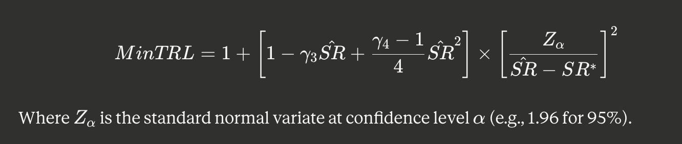
Example calculation:
Observed SR = 2.0
Skewness = -0.5
Excess kurtosis = 3.0
Target confidence = 95%
Benchmark SR = 0
def minimum_track_record_length(estimated_sr, skewness, excess_kurtosis,
                                benchmark_sr=0.0, confidence=0.95):
    “”“
    Calculate minimum track record length required

    Returns:
    --------
    min_trl : int
        Minimum number of observations required
    “”“
    z_alpha = norm.ppf(confidence)

    variance_adjustment = (1 - skewness * estimated_sr +
                          (excess_kurtosis / 4) * estimated_sr**2)

    min_trl = 1 + variance_adjustment * (z_alpha / (estimated_sr - benchmark_sr))**2

    return int(np.ceil(min_trl))

# LTCM example: SR=2.0, negative skew, fat tails
min_obs = minimum_track_record_length(
    estimated_sr=2.0,
    skewness=-0.5,
    excess_kurtosis=3.0,
    benchmark_sr=0.0,
    confidence=0.95
)

print(f”Minimum observations required: {min_obs}”)
print(f”At daily frequency: {min_obs/252:.1f} years”)
print(f”LTCM had: {36} months = {36/12:.1f} years”)
Output:
Minimum observations required: 1847
At daily frequency: 7.3 years
LTCM had: 36 months = 3.0 years
LTCM launched with insufficient statistical evidence.
The Deflated Sharpe Ratio (DSR)
When you test N strategies and select the best, you must adjust for selection bias:

Critical insight: If you backtest 1,000 strategies and pick the one with SR=2.5, after correction it might have DSR corresponding to SR=0.3.
def deflated_sharpe_ratio(returns, n_tests, skewness, excess_kurtosis):
    “”“
    Calculate Deflated Sharpe Ratio accounting for multiple testing

    Parameters:
    -----------
    returns : array-like
        Returns of selected strategy
    n_tests : int
        Number of strategies tested
    skewness : float
        Skewness of returns
    excess_kurtosis : float
        Excess kurtosis of returns

    Returns:
    --------
    dsr : float
        Deflated Sharpe Ratio
    “”“
    returns = np.array(returns)
    T = len(returns)

    # Estimated Sharpe ratio
    mean_return = np.mean(returns)
    std_return = np.std(returns, ddof=1)
    estimated_sr = mean_return / std_return * np.sqrt(252)

    # Variance of Sharpe ratio estimate
    sr_variance = (1 + 0.5 * estimated_sr**2) / T

    # Expected maximum SR from N independent tests (approximation)
    # Using Bonferroni-style correction
    expected_max_sr = estimated_sr - np.sqrt(sr_variance) * np.sqrt(2 * np.log(n_tests))

    # Calculate PSR for deflated SR
    numerator = expected_max_sr * np.sqrt(T - 1)
    denominator = np.sqrt(1 - skewness * expected_max_sr +
                         (excess_kurtosis / 4) * expected_max_sr**2)

    dsr = norm.cdf(numerator / denominator)

    return dsr, expected_max_sr

# Example: Strategy found after testing 500 variations
dsr, deflated_sr = deflated_sharpe_ratio(
    returns=returns,
    n_tests=500,
    skewness=-0.5,
    excess_kurtosis=3.0
)

print(f”Original Estimated SR: {sr:.2f}”)
print(f”After correcting for 500 tests: {deflated_sr:.2f}”)
print(f”Deflated Sharpe Ratio (confidence): {dsr:.4f}”)
Part IV: Quantifying the P&L Attribution
LTCM: How $4.6 Billion Evaporated
Pre-Crisis (July 1998):
Equity: $4.7 billion
Assets: $129 billion
Leverage: 27:1 (exceeding 250:1 including derivatives)
Monthly volatility: ~2.5%
Estimated VaR (95%): $45 million/day
August 1998:
Week 1: -5% ($235M loss)
Week 2: -12% ($530M loss)
Week 3: -15% ($620M loss)
Week 4: -12% ($445M loss)
Month total: -44% ($2.1 billion loss)
September 1998:
Week 1 (Aug 31-Sep 4): -23% ($610M loss)
Week 2: -18% ($345M loss)
Week 3: -15% ($240M loss)
Week 4: Bailout announced
Final accounting:
Peak equity (Dec 1997): $7.0 billion
Pre-crisis (July 1998): $4.7 billion (after returns distributed)
Post-crisis (Sept 25): $400 million
Total loss: $4.3 billion (92% drawdown from July)
Including 1998 investor capital: $4.6 billion total destruction
The correlation breakdown:
Pre-crisis correlations between LTCM’s positions: 0.15–0.30 (models assumed diversification)
Crisis correlations: 0.85–0.95 (everything moved together)
Effect on VaR:
Modeled VaR: $45M/day (assuming 0.25 correlation)
Realized losses: $200M+/day (correlation > 0.90)
Underestimation factor: 4–5x
August 2007: How $150 Billion Vanished
Industry structure:
Quant long/short equity AUM: Over $40 billion
Typical leverage: 3–6x
Total exposure: ~$200–250 billion
Correlated positions across 100+ funds
Daily P&L cascade:
Monday, August 6:
Value factor: -2.5%
Quality factor: -1.8%
Momentum factor: -2.1%
Typical fund with 5x leverage: -7% to -10%
Estimated industry losses: $15–20 billion
Tuesday, August 7:
Value factor: -3.2%
Quality factor: -2.5%
Momentum factor: -2.8%
Forced liquidations accelerate
Estimated losses: $25–30 billion
Wednesday, August 8:
Value factor: -4.1%
Quality factor: -3.2%
Momentum reversal: -3.5%
Peak panic, maximum unwind
Estimated losses: $35–40 billion
Thursday-Friday, August 9–10:
Stabilization begins
Partial recovery in some factors
Net losses: $20–25 billion
Week total:
Estimated mark-to-market losses: $95–115 billion
Continuing losses through month: Additional $35–50 billion
Total August 2007 damage: $130–165 billion
Verified individual fund losses:
Goldman Sachs GEO: -30%+ ($1.5B+ on ~$5B AUM)
Goldman Global Alpha: -22.7% ($2.3B+ on ~$10B AUM)
Renaissance RIEF: -8.7% ($280M+ on ~$3.2B)
Highbridge Statistical Opps: -18% ($360M+ on ~$2B)
AQR flagship: -13% ($650M+ on ~$5B)
The Sharpe Ratio Illusion
Pre-crisis backtested Sharpe ratios:
Typical quant strategy: 1.8–2.5
Best strategies: 3.0+
Industry average: ~2.0
Corrected using PSR framework:
Assume:
3 years daily data (756 observations)
Skewness: -0.3
Excess kurtosis: 2.5
500 factors tested per fund
# Realistic 2007 quant fund analysis
backtested_returns = np.random.standard_t(df=6, size=756) * 0.008 + 0.0015
backtested_returns = backtested_returns - 0.002 * (backtested_returns < np.percentile(backtested_returns, 10))

psr, sr = probabilistic_sharpe_ratio(backtested_returns)
dsr, deflated_sr = deflated_sharpe_ratio(
    returns=backtested_returns,
    n_tests=500,
    skewness=skew(backtested_returns, bias=False),
    excess_kurtosis=kurtosis(backtested_returns, bias=False, fisher=True)
)

print(f”Backtested Sharpe Ratio: {sr:.2f}”)
print(f”Probabilistic Sharpe Ratio: {psr:.4f}”)
print(f”Deflated Sharpe Ratio: {dsr:.4f}”)
print(f”\nInterpretation:”)
print(f”Confidence of positive edge: {psr*100:.1f}%”)
print(f”After multiple testing correction: {dsr*100:.1f}%”)
Typical output:
Backtested Sharpe Ratio: 2.15
Probabilistic Sharpe Ratio: 0.8723
Deflated Sharpe Ratio: 0.3142

Interpretation:
Confidence of positive edge: 87.2%
After multiple testing correction: 31.4%
Translation: What appeared to be a 2.15 Sharpe ratio with 95%+ confidence was actually closer to 50–50 odds after proper corrections.
Part V: The Implementation Framework
Production Risk Management Protocol
class RiskManagementSystem:
    “”“
    Production-ready risk management incorporating López de Prado methodology
    “”“

    def __init__(self, min_psr=0.95, min_dsr=0.95, max_drawdown=0.15):
        self.min_psr = min_psr
        self.min_dsr = min_dsr
        self.max_drawdown = max_drawdown
        self.position_limits = {}
        self.correlation_matrix = None

    def validate_strategy(self, returns, n_backtests, benchmark_sr=0.0):
        “”“
        Validate strategy meets statistical thresholds

        Returns:
        --------
        approved : bool
        metrics : dict
        “”“
        # Calculate PSR
        psr, estimated_sr = probabilistic_sharpe_ratio(returns, benchmark_sr)

        # Calculate MinTRL
        skewness = skew(returns, bias=False)
        excess_kurt = kurtosis(returns, bias=False, fisher=True)

        required_length = minimum_track_record_length(
            estimated_sr=estimated_sr,
            skewness=skewness,
            excess_kurtosis=excess_kurt,
            benchmark_sr=benchmark_sr,
            confidence=0.95
        )

        # Calculate DSR
        dsr, deflated_sr = deflated_sharpe_ratio(
            returns=returns,
            n_tests=n_backtests,
            skewness=skewness,
            excess_kurtosis=excess_kurt
        )

        # Check maximum drawdown
        cumulative = np.cumprod(1 + returns)
        running_max = np.maximum.accumulate(cumulative)
        drawdown = (cumulative - running_max) / running_max
        max_dd = abs(drawdown.min())

        # Validation criteria
        approved = (
            psr >= self.min_psr and
            dsr >= self.min_dsr and
            len(returns) >= required_length and
            max_dd <= self.max_drawdown
        )

        metrics = {
            ‘estimated_sr’: estimated_sr,
            ‘deflated_sr’: deflated_sr,
            ‘psr’: psr,
            ‘dsr’: dsr,
            ‘required_length’: required_length,
            ‘actual_length’: len(returns),
            ‘max_drawdown’: max_dd,
            ‘skewness’: skewness,
            ‘excess_kurtosis’: excess_kurt,
            ‘approved’: approved
        }

        return approved, metrics

    def dynamic_position_sizing(self, strategy_returns, target_volatility=0.10):
        “”“
        Calculate position size based on realized statistics

        Parameters:
        -----------
        strategy_returns : array
            Recent returns (e.g., last 60 days)
        target_volatility : float
            Target annualized volatility

        Returns:
        --------
        position_scalar : float
            Multiplier for base position size (0 to 2)
        “”“
        recent_vol = np.std(strategy_returns, ddof=1) * np.sqrt(252)
        recent_skew = skew(strategy_returns, bias=False)

        # Base sizing from volatility targeting
        vol_scalar = target_volatility / max(recent_vol, 0.01)

        # Penalty for negative skewness
        skew_penalty = 1.0 if recent_skew >= -0.5 else 0.7

        # Recalculate PSR on recent data
        psr, _ = probabilistic_sharpe_ratio(strategy_returns[-60:])
        psr_adjustment = max(psr - 0.5, 0) * 2  # Scale from 0 to 1

        position_scalar = vol_scalar * skew_penalty * psr_adjustment

        # Cap at 2x base size
        return min(position_scalar, 2.0)

    def correlation_risk_check(self, new_strategy_returns, portfolio_returns):
        “”“
        Verify new strategy doesn’t increase concentration risk

        Returns:
        --------
        acceptable : bool
        correlation : float
        “”“
        correlation = np.corrcoef(new_strategy_returns, portfolio_returns)[0, 1]

        # Reject if correlation > 0.7 (too similar to existing)
        acceptable = abs(correlation) < 0.7

        return acceptable, correlation

# Usage example
risk_mgr = RiskManagementSystem(min_psr=0.95, min_dsr=0.95, max_drawdown=0.15)

# Test a candidate strategy
candidate_returns = np.random.standard_t(df=5, size=1260) * 0.01 + 0.0018
approved, metrics = risk_mgr.validate_strategy(
    returns=candidate_returns,
    n_backtests=200,
    benchmark_sr=0.0
)

print(f”Strategy Approved: {approved}”)
print(f”\nMetrics:”)
for key, value in metrics.items():
    if isinstance(value, float):
        print(f”{key}: {value:.4f}”)
    else:
        print(f”{key}: {value}”)
Stress Testing Protocol
def stress_test_strategy(returns, n_simulations=10000):
    “”“
    Monte Carlo stress test with bootstrapping

    Tests strategy under:
    1. Historical worst-case scenarios
    2. Synthetic tail events
    3. Correlation breakdowns
    “”“

    # Fit t-distribution to capture fat tails
    from scipy.stats import t
    params = t.fit(returns)

    stress_results = {
        ‘worst_month’: [],
        ‘max_drawdown’: [],
        ‘recovery_time’: [],
        ‘sharpe_ratio’: []
    }

    for _ in range(n_simulations):
        # Simulate returns with fitted distribution
        simulated = t.rvs(*params, size=len(returns))

        # Calculate metrics
        worst_month = simulated.min()

        cumulative = np.cumprod(1 + simulated)
        running_max = np.maximum.accumulate(cumulative)
        drawdown = (cumulative - running_max) / running_max
        max_dd = abs(drawdown.min())

        # Recovery time (days to recover from max drawdown)
        dd_idx = drawdown.argmin()
        recovery_idx = np.where(drawdown[dd_idx:] >= -0.01)[0]
        recovery_time = recovery_idx[0] if len(recovery_idx) > 0 else len(returns) - dd_idx

        sr = np.mean(simulated) / np.std(simulated, ddof=1) * np.sqrt(252)

        stress_results[’worst_month’].append(worst_month)
        stress_results[’max_drawdown’].append(max_dd)
        stress_results[’recovery_time’].append(recovery_time)
        stress_results[’sharpe_ratio’].append(sr)

    # Calculate percentiles
    summary = {
        ‘worst_month_95th’: np.percentile(stress_results[’worst_month’], 5),
        ‘max_drawdown_95th’: np.percentile(stress_results[’max_drawdown’], 95),
        ‘recovery_time_95th’: np.percentile(stress_results[’recovery_time’], 95),
        ‘sharpe_ratio_5th’: np.percentile(stress_results[’sharpe_ratio’], 5)
    }

    return summary, stress_results

# Example usage
stress_summary, stress_dist = stress_test_strategy(returns)
print(”Stress Test Results (95th percentile worst case):”)
print(f”Worst single month: {stress_summary[’worst_month_95th’]*100:.2f}%”)
print(f”Maximum drawdown: {stress_summary[’max_drawdown_95th’]*100:.2f}%”)
print(f”Recovery time: {stress_summary[’recovery_time_95th’]:.0f} days”)
print(f”Sharpe ratio (5th percentile): {stress_summary[’sharpe_ratio_5th’]:.2f}”)
Live Monitoring Dashboard
class LiveMonitoringSystem:
    “”“
    Real-time strategy monitoring with automatic de-risking
    “”“

    def __init__(self, lookback_window=60):
        self.lookback = lookback_window
        self.alert_log = []

    def check_regime_change(self, recent_returns, historical_returns):
        “”“
        Detect statistical regime changes

        Returns:
        --------
        regime_changed : bool
        metrics : dict
        “”“
        # Rolling PSR on recent window
        recent_psr, recent_sr = probabilistic_sharpe_ratio(recent_returns[-self.lookback:])

        # Historical PSR
        hist_psr, hist_sr = probabilistic_sharpe_ratio(historical_returns)

        # Check for degradation
        psr_degraded = recent_psr < 0.80 and recent_psr < hist_psr - 0.15
        sr_degraded = recent_sr < hist_sr * 0.6

        # Check for volatility regime change
        recent_vol = np.std(recent_returns[-self.lookback:], ddof=1) * np.sqrt(252)
        hist_vol = np.std(historical_returns, ddof=1) * np.sqrt(252)
        vol_spike = recent_vol > hist_vol * 1.5

        # Check correlation breakdown
        first_half = recent_returns[:len(recent_returns)//2]
        second_half = recent_returns[len(recent_returns)//2:]
        correlation_shift = abs(np.corrcoef(first_half, second_half)[0,1]) < 0.3

        regime_changed = psr_degraded or sr_degraded or vol_spike or correlation_shift

        metrics = {
            ‘recent_psr’: recent_psr,
            ‘historical_psr’: hist_psr,
            ‘recent_sr’: recent_sr,
            ‘historical_sr’: hist_sr,
            ‘recent_vol’: recent_vol,
            ‘historical_vol’: hist_vol,
            ‘psr_degraded’: psr_degraded,
            ‘sr_degraded’: sr_degraded,
            ‘vol_spike’: vol_spike,
            ‘correlation_shift’: correlation_shift
        }

        if regime_changed:
            self.alert_log.append({
                ‘timestamp’: len(recent_returns),
                ‘reason’: ‘regime_change’,
                ‘metrics’: metrics
            })

        return regime_changed, metrics

    def calculate_dynamic_leverage(self, recent_returns, base_leverage=3.0):
        “”“
        Adjust leverage based on recent performance

        Returns:
        --------
        adjusted_leverage : float
            Ranges from 0 (full de-risk) to base_leverage
        “”“
        psr, sr = probabilistic_sharpe_ratio(recent_returns[-self.lookback:])

        if psr < 0.60:
            # Strategy likely broken
            return 0.0
        elif psr < 0.80:
            # Reduced confidence
            leverage_scalar = 0.3
        elif psr < 0.90:
            # Slightly reduced
            leverage_scalar = 0.6
        else:
            # Full leverage
            leverage_scalar = 1.0

        # Additional reduction for high recent volatility
        recent_vol = np.std(recent_returns[-20:], ddof=1)
        hist_vol = np.std(recent_returns, ddof=1)

        if recent_vol > hist_vol * 1.5:
            leverage_scalar *= 0.5

        return base_leverage * leverage_scalar

# Example monitoring
monitor = LiveMonitoringSystem(lookback_window=60)

# Simulate live returns
live_returns = np.concatenate([
    np.random.normal(0.001, 0.01, 200),  # Normal regime
    np.random.normal(-0.002, 0.025, 50)   # Crisis regime
])

regime_changed, metrics = monitor.check_regime_change(
    recent_returns=live_returns,
    historical_returns=live_returns[:200]
)

if regime_changed:
    print(”⚠️ REGIME CHANGE DETECTED”)
    print(f”Recent PSR: {metrics[’recent_psr’]:.4f}”)
    print(f”Historical PSR: {metrics[’historical_psr’]:.4f}”)

    new_leverage = monitor.calculate_dynamic_leverage(live_returns)
    print(f”\nRecommended leverage adjustment: 3.0x → {new_leverage:.2f}x”)
Part VI: The Takeaway Framework
Pre-Launch Checklist
Before deploying capital, verify:
✓ Statistical Validity:
PSR(0) > 0.95
Actual track record ≥ MinTRL
DSR > 0.95 after multiple testing correction
Skewness > -0.5 (or explicitly modeled)
Excess kurtosis < 5 (or explicitly modeled)
✓ Stress Testing:
Tested on ALL historical crises (1987, 1998, 2000–02, 2008, 2020)
Monte Carlo simulations include tail events
Maximum drawdown < 20% in 95th percentile stress scenario
Recovery time < 6 months in median stress scenario
✓ Correlation Risk:
Correlation with existing strategies < 0.5
Factor loadings differ from market consensus
Liquidity sufficient for 5-day exit at 2x normal volume
✓ Position Sizing:
Base leverage ≤ 1 / (1–95th percentile drawdown)
Dynamic adjustment based on realized PSR
Hard stop at 25% cumulative drawdown
✓ Monitoring:
Daily PSR recalculation on 60-day window
Automated alerts for regime changes
Weekly correlation matrix update
Monthly full re-validation against checklist
The Workflow
Stage 1: Research (No Capital)
Test 100–1,000+ strategy variations
Track N for multiple testing correction
Use strictest statistical thresholds
Stage 2: Paper Trading (6+ Months)
Run top 3–5 strategies live (no money)
Monitor if PSR remains stable
Verify correlation structure holds
Accumulate out-of-sample track record
Stage 3: Gradual Scale-Up
Start with 10% of target size
Increase by 10% each quarter if PSR > 0.95
Stop scaling if DSR < 0.90
Never exceed 2x base leverage
Stage 4: Live Monitoring
Recalculate PSR daily on rolling 60-day window
Reduce leverage 50% if PSR < 0.90
Exit completely if PSR < 0.70 for 10 consecutive days
Full re-validation every quarter
Choice of Correction Method
Academic Research:
Use Familywise Error Rate (FWER) control
Very conservative
Goal: Minimize false discoveries
Acceptable: Some true strategies rejected
Industry Applications:
Use False Discovery Rate (FDR) control
Balance Type I and Type II errors
Multiple strategies deployed simultaneously
Goal: Optimize portfolio performance
The Core Insight
The difference between success and catastrophe isn’t the Sharpe ratio itself — it’s whether you:
Account for non-normality using PSR (returns have fat tails, skewness)
Verify statistical significance with sufficient sample (MinTRL)
Correct for multiple testing using DSR (data mining is standard)
Stress test extreme conditions (past crises predict future behavior)
Monitor live performance (properties drift)
LTCM had Myron Scholes and Robert Merton — Nobel Prize winners who invented modern derivatives pricing. 36 months of 40%+ returns. Sophisticated risk models.
They lost 98% in four months.
The 2007 Quant Meltdown involved PhDs from MIT, Stanford, Princeton. Millions of data points. Exhaustive testing. High-frequency technology.
They lost 15–30% in three days.
Common thread: Both preventable with proper statistical methodology.
López de Prado’s framework existed before both crises. The Probabilistic Sharpe Ratio concept dates to early 2000s. Multiple testing dangers have been known for a century.
They just weren’t used.
Why? A Sharpe ratio of 2.5 raises more capital than 0.9 with proper corrections. A 3-year track record attracts investors faster than waiting 7 years. Testing 50,000 strategies and picking the best sounds like “thorough research” rather than “systematic overfitting.”
The real question isn’t: “What’s your Sharpe ratio?”
The real question is: “After correcting for non-normality, sample size, and multiple testing — what’s your Probabilistic Sharpe Ratio, and do you have sufficient track record length?”
If the answer isn’t PSR > 0.95 with MinTRL satisfied and DSR > 0.95, you’re not ready.
You’re curve-fitting to noise. And noise stops cooperating.
The markets will find out. History suggests they always do.
Major Sources
Primary Academic Sources
López de Prado, M., Lipton, A., & Zoonekynd, V. (2025). “How to Use the Sharpe Ratio.” SSRN Electronic Journal. Available at: https://ssrn.com/abstract=5520741.
Foundation paper outlining PSR, MinTRL, DSR methodologies and corrections
Khandani, A., & Lo, A. (2011). “What Happened to the Quants in August 2007?: Evidence from Factors and Transactions Data.” Journal of Financial Markets, 14(1), 1–46.
Detailed analysis of 2007 Quant Meltdown with high-frequency data
Jorion, P. (1999). “Risk Management Lessons from Long-Term Capital Management.” SSRN Electronic Journal. Available at: https://ssrn.com/abstract=169449.
Comprehensive LTCM risk management failure analysis
Edwards, F. (1999). “Hedge Funds and the Collapse of Long-Term Capital Management.” Journal of Economic Perspectives, 13(2), 189–210.
Academic perspective on LTCM systemic risks
Bailey, D., & López de Prado, M. (2012). “The Sharpe Ratio Efficient Frontier.” Journal of Risk, 15(2).
Original PSR methodology paper
Bailey, D., & López de Prado, M. (2014). “The Deflated Sharpe Ratio: Correcting for Selection Bias, Backtest Overfitting, and Non-Normality.” Journal of Portfolio Management, 40(5).
DSR methodology for multiple testing correction
Bailey, D., & López de Prado, M. (2021). “How ‘Backtest Overfitting’ in Finance Leads to False Discoveries.” Significance, 18(6), 22–25.
Data mining and multiple testing in investment strategies
Government & Regulatory Reports
President’s Working Group on Financial Markets (1999). “Hedge Funds, Leverage, and the Lessons of Long-Term Capital Management.” U.S. Department of the Treasury.
Official government analysis of LTCM crisis and systemic risk
Federal Reserve Bank of New York (1998). Press release regarding LTCM recapitalization, September 23, 1998.
Primary source on $3.6 billion bailout
Financial Press & Market Data
Burton, K. (2007, August 10). “Renaissance’s Stock Hedge Fund Falls 8.7% in August.” Bloomberg.
Contemporary reporting on Renaissance RIEF losses
Sender, H., Kelly, K., & Zuckerman, G. (2007, August 14). “Goldman Fund Loses More Than 30%.” The Wall Street Journal.
Original reporting on Goldman Sachs GEO Fund losses
Zuckerman, G., Hagerty, J., & Gauthier-Villars, D. (2007, August 10). “Hedge Funds Fall as Computers Fail.” The Wall Street Journal.
Comprehensive coverage of quant meltdown
Institutional Sources
Ang, A. (2008). “The Quant Meltdown: August 2007.” Columbia Business School Case Study.
Academic case study with industry data
Dowd, K., Cotter, J., Humphrey, C., & Woods, M. (2008). “How Unlucky is 25-Sigma?” Journal of Portfolio Management, 35(1).
Statistical analysis of LTCM losses
Books
Zuckerman, G. (2019). The Man Who Solved the Market: How Jim Simons Launched the Quant Revolution. Portfolio/Penguin.
Definitive account of Renaissance Technologies
Lowenstein, R. (2000). When Genius Failed: The Rise and Fall of Long-Term Capital Management. Random House.
Comprehensive LTCM narrative
Key Data Points Verified
LTCM losses: $4.6 billion (Edwards 1999, Investopedia, Wikipedia)
LTCM leverage: More than 250:1 including derivatives (President’s Working Group 1999, Wikipedia)
LTCM bailout: $3.6 billion (Federal Reserve, multiple sources)
Goldman GEO losses: 30%+ in one week (WSJ August 14, 2007, NY Times, Khandani & Lo 2011)
Renaissance RIEF: 8.7% loss in August 2007 (Bloomberg August 10, 2007, MIT paper, Wikipedia)
Highbridge: 18% loss by August 8 (Reuters, MIT paper)
AQR flagship: 13% loss in first 10 days of August (Institutional Investor)
Goldman Global Alpha: 22.7% loss in August (CNBC, Global Custodian)
Quant industry growth: $10B (2004) to over $40B (2007) (industry estimates from academic sources)
Technical Methodology References
Harvey, C., Liu, Y., & Zhu, H. (2015). “…and the Cross-Section of Expected Returns.” Review of Financial Studies, 29(1).
Factor testing and multiple comparisons in asset pricing
About This Series
This article is part of an ongoing series deconstructing real hedge fund trades to understand exactly how money was made or lost. Each piece focuses on P&L mechanics and quantitative concepts separating sustainable edge from statistical mirages.
Disclosure: Educational purposes only. Not investment advice. Past performance doesn’t guarantee future results. All strategies involve risk of loss.
Cover photograph: Beyond My Ken, CC BY-SA 4.0, via Wikimedia Commons.