


This is a detailed research piece. If you find value in institutional-quality hedge fund analysis, support this work on Patreon.

Investment banks generate returns by exploiting systematic mispricing between index and single-stock options through dispersion trading — a correlation arbitrage strategy that achieved 14.52–26.51% annual returns with Sharpe ratios of 0.34–0.40 in backtests on S&P 500 constituents from January 2000 to December 2017, though earlier studies documented profitability declines post-2000 requiring refined execution methods.
The Setup: Structural Mispricing in Option Markets
Index options embed systematically higher implied correlation than realized correlation. While index implied volatility (IV) is mathematically lower than component IVs due to diversification, the implied correlation backing out from index option prices consistently exceeds realized correlation between stocks — creating a tradeable correlation risk premium.
This mispricing stems from asymmetric demand flows. Institutional investors hedge portfolio risk by purchasing index puts, driving up index IV relative to its theoretical value derived from component volatilities. Simultaneously, portfolio managers sell single-stock covered calls to enhance returns, suppressing component IVs. Banks like J.P. Morgan, Morgan Stanley, and Goldman Sachs monetize the gap between implied correlation (priced into expensive index options) and realized correlation (actual co-movement of stocks).
Trade Structure: Long Component Volatility, Short Index Volatility
The canonical dispersion trade involves three positions executed simultaneously:
Sell index options (typically ATM straddles on S&P 500 or sector indices)
Buy options on index constituents (weighted ATM straddles matching index composition)
Delta-hedge the entire portfolio (maintain market-neutral exposure)
Position sizing follows precise mathematical constraints. For a gamma-flat dispersion trade, basket weights are calibrated such that the gamma exposure of the short index position offsets the long gamma from component options. This requires solving:
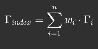
where $w_i$ represents the optimal weight for stock $i$, typically determined through principal component analysis to maximize explanatory power while minimizing basket size.
P&L Mechanics: Harvesting the Correlation Premium
Profitability derives from the spread between realized and implied correlation. When individual stocks disperse (low realized correlation), the long component options capture movement while the short index position decays as index volatility remains subdued.
Consider a simplified example: Stock A drops 10%, Stock B rallies 10%, while the index remains unchanged. The trader collects:
Premium from short index straddle (expires worthless: +6% notional)
Payoffs from long component straddles: 0.5×10% + 0.5×10% = 10% gross movement
Premium cost for component straddles: -8.5% (components trade with lower IV individually)
Net P&L: +6% (index) + 1.5% (components net) = +7.5% on notional
The strategy’s expected return decomposes into (Jacquier & Slaoui, 2010):

where the first term captures pure correlation arbitrage and the Volga term reflects second-order convexity effects.
Risk Management: Delta-Hedging and Rebalancing Discipline
Maintaining delta-neutrality requires intraday rebalancing as underlying prices move. Sell-side desks employ automated delta hedging systems that:
Monitor aggregate portfolio delta continuously
Execute offsetting trades in underlying stocks or futures when delta breaches predefined bands (typically ±0.01–0.05% of notional)
Minimize transaction costs through optimal execution algorithms
Transaction costs significantly impact net returns. Schneider & Stübinger (2020) demonstrated that unhedged dispersion achieved 26.51% annual returns versus 14.52% for delta-hedged variants — about a 12 percentage point performance gap, largely attributable to hedging and transaction costs in their 2000–2017 S&P 500 study. Sophisticated desks mitigate this through:
Optimized stock selection (using PCA to reduce basket size from 500 to 30–50 stocks)
Wider delta bands during low-volatility regimes
Leveraging internal flow to offset client hedging needs
Performance Drivers and Market Regime Dependence
Empirical evidence from S&P 500 dispersion trades (2000–2017) demonstrates:
Base case returns: 14.52% p.a. (delta-hedged), 26.51% p.a. (unhedged)
Sharpe ratios: 0.34–0.40
Critical context: Early research documented exceptional profitability in Deng’s 1996–2000 sample (monthly returns of 24% with Sharpe 1.2), but returns declined substantially post-2000, with some studies showing negative performance. The Schneider & Stübinger results (2000–2017) represent a recovery period with refined selection methods.
Worst drawdowns: During 2008–2009 Financial Crisis, realized correlation spiked as stocks moved in lockstep, causing significant losses for short correlation positions. March 2020 COVID crash (outside the 2000–2017 sample) produced similar correlation-driven losses.
The strategy exhibits negative skewness — small consistent gains punctuated by tail losses during market stress. Banks structure exposure accordingly:
Reduce notional during high-volatility regimes when correlations typically rise
Use implied correlation indices (CBOE ICJ) as timing signals
Layer on tail hedges through out-of-the-money index put spreads
BNP Paribas research identifies three tradeable profiles:
Gamma-flat: Captures correlation premium with minimal directional exposure; most defensive profile
Vega-flat: Isolates pure correlation bets, immune to parallel volatility shifts across all strikes
Theta-flat: Trades correlation with minimized time decay; higher positive carry in bull markets
Market Sizing and Institutional Context
Dispersion trades in equity indices reached approximately $3–5 million vega notional daily by the mid-2000s (JPMorgan European Equity Derivatives Strategy, 2006), growing as banks sought flow-based revenue post-crisis. Morgan Stanley, J.P. Morgan, and Deutsche Bank dominate European equity derivatives markets with material dispersion franchises. Goldman Sachs and Bank of America lead in North American flow options, where dispersion strategies complement structured product issuance.
QIS (Quantitative Investment Strategies) products now package dispersion trades as swaps or structured notes for institutional clients, enabling pension funds and family offices to access systematic correlation premium without operational complexity. This sell-side productization has expanded dispersion product availability across multiple asset managers, with individual funds typically managing assets in the hundreds of millions range.
Key Takeaway
Dispersion trading exemplifies how sell-side quants monetize persistent behavioral biases in option markets. By systematically selling overpriced index correlation and buying underpriced component volatilities — while maintaining rigorous delta-neutrality — banks extract consistent alpha from structural supply-demand imbalances. Success requires sophisticated position construction, ruthless transaction cost management, and disciplined risk controls to survive inevitable correlation spikes during market dislocations.
Sources
Academic Research:
Schneider, L. & Stübinger, J. (2020). “Dispersion Trading Based on the Explanatory Power of S&P 500 Stock Returns.” Mathematics, 8(9), 1627. https://www.mdpi.com/2227-7390/8/9/1627
Marshall, C.M. (2009). “Dispersion trading: Empirical evidence from U.S. options markets.” Global Finance Journal, 20(3), 289–301. https://ideas.repec.org/a/eee/glofin/v20y2009i3p289-301.html
Deng, Q. (2008). “Volatility Dispersion Trading.” SSRN Working Paper. https://papers.ssrn.com/sol3/papers.cfm?abstract_id=1156620
Jacquier, A. & Slaoui, S. (2010). “Variance Dispersion and Correlation Swaps.” Birkbeck Working Papers, BBKEFP 0712.
https://ideas.repec.org/p/bbk/bbkefp/0712.html
Ferrari, P., Poy, G., & Abate, G. (2019). “Dispersion trading: an empirical analysis on the S&P 100 options.” Investment Management and Financial Innovations, 16(1), 178–188. https://businessperspectives.org/journals/investment-management-and-financial-innovations/issue-321/dispersion-trading-an-empirical-analysis-on-the-s-p-100-options
Industry Research:
BNP Paribas QIS Lab. “Equity Dispersion: how, what and when to trade.” BNP Paribas Global Markets. https://globalmarkets.cib.bnpparibas/equity-dispersion-trading/
JPMorgan (2006). “Just what you need to know about Variance Swaps.” European Equity Derivatives Strategy. https://derivativesacademy.com/storage/uploads/files/modules/resources/1702207867_allen_einchcomb_granger_jpm_2006_variance_swaps.pdf
STOXX (2024). “An Index Solution for Dispersion Trading.” STOXX Indices Research. https://stoxx.com/an-index-solution-dispersion-trading/
Greenwich Associates (2013). “Flow Equity Derivatives Market Study.” https://www.greenwich.com/press-release/flow-equity-derivatives-morgan-stanley-most-widely-used-broker-europe-goldman-sach
Institutional Sources:
Cboe Global Markets. “S&P 500 Implied Correlation Index (ICJ).” CBOE Index Documentation. https://cdn.cboe.com/resources/indices/documents/impliedcorrelationindicator.pdf
Quantpedia (2024). “Dispersion Trading Strategy Analysis.” https://quantpedia.com/strategies/dispersion-trading
BSIC Bocconi (2024). “Backtesting Dispersion Trading Chapter I.” https://bsic.it/backtesting-dispersion-trading-chapter-i/
CQF Institute. “What is Dispersion trading?” https://www.cqf.com/blog/quant-finance-101/what-is-dispersion-trading
📊 Support this research: https://www.patreon.com/c/NavnoorBawa
Cover photograph: Kidfly182, CC BY 4.0, via Wikimedia Commons.
That 12 percentage point gap between hedged and unhedged returns really puts transaction costs into perspective. You basically pay half your alpha just to keep the position delta neutral, which makes sense when you're constantly rebalancing across 50+ names.