



D.E. Shaw, Citadel, and Renaissance are among the largest practitioners of statistical arbitrage, running mean-reversion strategies on the Ornstein-Uhlenbeck framework that has been the field standard since Avellaneda and Lee’s 2010 paper. That framework carries an OLS estimation bias in its core mean-reversion parameter documented in Biometrika since 1954, and the Avellaneda-Lee paper that established the standard does not address it. The dominant explanation for declining statistical arbitrage alpha is crowding: more capital chasing fewer structural mispricings, signal half-life compressed, position correlations rising until forced liquidation triggers cascade losses. That story is right about the facts and incomplete about the mechanism. A second, causally distinct error runs in parallel: OLS estimation of κ in the discretized Ornstein-Uhlenbeck process is finite-sample biased by an order inversely proportional to the calendar span T of the estimation window, not the sample size n. A fund shifting from daily to hourly sampling over the same 60-day window reduces this error by exactly zero. At the Avellaneda and Lee (2010) standard of T₁ = 60 trading days, the Marriott-Pope bias drives calibrated half-lives below their true values, causing funds to trigger exits while the majority of the spread deviation remains open. How large this error is relative to crowding-driven signal decay is not quantifiable from public data. What is established is the mechanism: it exists, it has a known structure, and the fix is available.
The Consensus and the Layer Beneath It
The standard account is empirically grounded. Gatev, Goetzmann and Rouwenhorst (2006) documented average annualized excess returns of up to 11% for the top pairs portfolios over 1962–2002, measured after controlling for bid-ask bounce via a one-day delay but before explicit commissions; the paper states that profits “typically exceed conservative transaction-cost estimates.” Do and Faff (2010) showed, using CRSP data from 1962–2009, that pairs trading profitability was strongest in the period before 1989 and declined from the 1990s onward; a finding widely attributed to their paper across independent academic replications, though the paper’s abstract describes only “the continuing downward trend” without sub-period labels. McLean and Pontiff (2016) showed that across 97 cross-sectional return predictors (a broad sample that includes factor-based strategies but not specifically OU stat arb), portfolio returns were 26% lower out-of-sample (the paper describes this as “an upper bound estimate of data mining effects”) and 58% lower post-publication, with an estimated 32% decline attributable to publication-informed trading. Applying this to OU stat arb is an inference, not a direct measurement.
That account explains erosion of the SIGNAL: the statistical relationship between spread deviation and subsequent convergence. It does not explain errors in how that signal is PROCESSED after entry. A fund that correctly identifies a profitable spread, correctly enters, and exits at the wrong time loses alpha from an implementation failure that is causally separate from crowding, unaffected by how many other funds are in the same trade. These two loss sources have different mechanisms and different remedies. How much each contributes to observed Sharpe compression cannot be resolved from publicly available data.
The Avellaneda-Lee Estimation Architecture
Avellaneda and Lee decompose individual stock returns into a systematic component, explained by sector ETFs or principal components, and an idiosyncratic residual dXᵢ, modeled as:

All three parameters are estimated from a rolling 60-day window (T₁ = 60/252 ≈ 0.238 calendar years). The paper states entry at any residual that deviates by 1.25 standard deviations from equilibrium, and exit when the residual is less than 0.5 standard deviations from equilibrium, a threshold specified uniformly across all stocks. The tradeability filter requires κᵢ > 252/30 = 8.4 per year (half-life under 30 trading days).
From κ̂ᵢ flows every quantity that matters operationally: the S-score
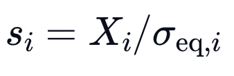

The position size, and the tradeability filter. If κ̂ is materially wrong, all of them are wrong simultaneously.
The paper covers 1997–2007. PCA-based strategies averaged Sharpe 1.44 over that full window, a figure that already incorporates the weak later years; during 2003–2007 alone, the sub-period Sharpe was only 0.9. The paper describes pre-2003 performance as “much stronger” without reporting the sub-period separately. Working backward from the stated averages: if the full 11-year average is 1.44 and the 2003–2007 (5-year) average is 0.9, the implied 1997–2002 (6-year) average is approximately 1.89, meaning the within-sample drop was from roughly 1.89 to 0.9. Post-2010 performance of the vanilla OLS implementation is unobservable from public primary sources.
The T⁻¹ Bias: Mechanism and Lineage
The finite-sample bias in AR coefficient estimation was first formally analyzed by Hurwicz (1950) in the Cowles Commission Monograph on dynamic economic models. Marriott and Pope (1954) derived the first analytical approximation in Biometrika: for an AR(1) with intercept, the OLS estimate of the autoregressive coefficient â₁ is biased by approximately −(1 + 3a₁)/n. That discrete-time result sat in the econometrics literature for 55 years before Tang and Chen (2009) adapted it to the continuous-time OU process in the Journal of Econometrics, establishing that the bias in κ̂ is of order T⁻¹ (total calendar span), not n⁻¹ (sample size). Yu (2012) refined the formula with a nonlinear correction, identifying that the Marriott-Pope approximation “does not work satisfactorily when the speed of mean reversion is slow”: the near-unit-root regime, because in that limit, Yu showed, “the true bias has an interesting curvature and goes to zero when the mean reversion parameter is closer to zero.” This correction matters for the worked examples below.
The T⁻¹ vs. n⁻¹ result is the operationally decisive finding. A fund sampling daily over 60 days (n = 60, T = 0.238 years) faces bias of order 1/T ≈ 4.2 per year. The same fund sampling hourly (n = 1,260, T unchanged) faces the same bias. Only extending the window to 120 days halves it.
The Marriott-Pope Cascade: What the First-Order Approximation Shows
When practitioners estimate κ by regressing Xₜ₊₁ on Xₜ and a constant to obtain â₁, then computing κ̂ = −ln(â₁)/Δt, the Marriott-Pope bias in â₁ (toward zero) translates into an upward bias in κ̂:
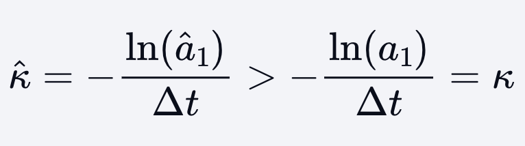
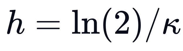
Mean-reversion appears faster than it is. The estimated half-life
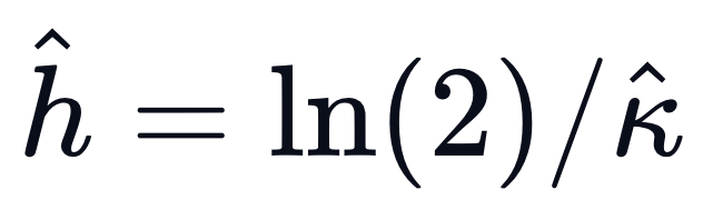
falls below the true half-life.
The calculations below use the first-order Marriott-Pope approximation, Bias(â₁) ≈ −(1+3a₁)/n. This approximation is more reliable away from unit root and deteriorates as a₁ approaches 1. In the near-unit-root case (the κ = 3.8 example, where a₁ ≈ 0.985), Yu (2012) shows the true bias is actually smaller than Marriott-Pope predicts, because the true bias in κ approaches zero as κ approaches zero. That example should be read as an upper bound on the bias magnitude in that regime, not a point estimate. The κ = 15 example, where a₁ ≈ 0.942, is less affected by this limitation and is the more reliable illustration.
For a pair with true κ = 15/year (true half-life ≈ 11.6 trading days):
Daily AR coefficient: a₁ = e^{−15/252} ≈ 0.942
Marriott-Pope bias: −(1 + 3 × 0.942)/60 ≈ −0.064; estimated â₁ ≈ 0.878
κ̂ ≈ 33.0/year (120% above true κ under this approximation)
Estimated half-life ≈ 5.3 trading days (vs. true 11.6)
For a pair with true κ = 3.8/year (true half-life ≈ 46 trading days), in the near-unit-root regime where Marriott-Pope overstates the bias:
a₁ = e^{−3.8/252} ≈ 0.985; estimated â₁ ≈ 0.919 under Marriott-Pope
κ̂ ≈ 21.3/year under this approximation; this pair would pass the κ > 8.4 filter
The 460% overstatement derived from Marriott-Pope is an upper bound; the true magnitude requires Yu’s numerical formula
What the two cases illustrate mechanistically: a pair that should fail the tradeability filter (true half-life 46 days, which is outside the intended < 30-day screen) can pass it because biased κ estimation makes it look fast. And a pair that is truly fast-reverting gets assigned an estimated half-life that is a fraction of the true value, causing the exit signal to fire before most of the convergence has occurred.
The fraction of reversion remaining at the biased exit point (first-order approximation):

For κ = 15, κ̂ = 33 (the more reliable example): 2^{−15/33} ≈ 0.73 under this approximation. This illustrates that if the approximation holds, the exit signal fires while roughly 73% of the spread deviation remains open.
These are derived quantities from a first-order formula applied to chosen illustrative parameters, not measurements from any live book. Their value is in showing that the mechanism, if present, would not be a small second-order effect; even under a conservative approximation, the bias ratio κ̂/κ ≈ 2 is large enough to matter. Whether it matters as much as crowding in any specific implementation is unresolvable from public data.
The Standard Error Reinforces the Same Conclusion
For κ = 15/year with 60 daily observations, the standard error of κ̂ from the AR(1) regression via delta method is approximately SE(κ̂) ≈ 252 × √((1−a₁²)/n) / a₁ ≈ 11.9 per year.
Centered on the true κ = 15, the 95% interval for what an analyst would observe spans roughly [−8, 38] per year, essentially uninformative about whether the true half-life is 5 days or 60 days. Centered on the observable κ̂ ≈ 33 (the only value an analyst actually has in production), the interval spans roughly [10, 56] per year, still wide enough to be consistent with the true κ ranging from near-zero to very fast reversion. Both framings point to the same conclusion: the 60-day window cannot reliably identify the parameter that governs every downstream exit decision.
Crowding Is a Bias Amplifier, Not the Primary Source
When multiple funds hold identical long-short positions, their collective flow physically accelerates convergence, raising the realized κ in the estimation window. A fund running 60-day OLS calibrates to this crowding-inflated speed and sizes up accordingly.
When any fund begins to liquidate (the “Unwind Hypothesis” of Khandani and Lo, NBER Working Paper 14465 (2008)), the coordinated flow stops. Remaining funds are positioned to a κ that only existed under crowded conditions.
Khandani and Lo found in the NBER paper that “the expected return of a simple mean-reversion strategy increased monotonically with the holding period during this time, i.e., those marketmakers that were able to hold their positions longer received higher premiums.” Two limitations apply when invoking this as evidence for the bias-exit thesis: first, the strategy they simulated is the Lehmann (1990)/Lo-MacKinlay (1990) daily contrarian, not the Avellaneda-Lee OU approach; the holding-period premium is consistent with the early-exit mechanism but is not a test of it. Second, Khandani and Lo explicitly state that “the hypotheses advanced in this paper are speculative, tentative, and based solely on indirect evidence”; they had no access to fund-level position data. The inference chain from that paper to the bias-exit mechanism requires multiple steps, each of which adds uncertainty.
Decay and Capacity: What the Mechanism and What the Unknowns Are
The underlying signal (idiosyncratic mean-reversion after factor neutralization) is subject to publication-informed decay. Applying the McLean-Pontiff framework by inference, with the caveat that their study covers cross-sectional predictors broadly rather than OU stat arb specifically, the GGR publication in 2006 likely accelerated capital flows into the strategy. The within-sample degradation Avellaneda and Lee document is consistent with that trend: from a pre-2003 implied Sharpe of roughly 1.89 to 0.9 in 2003–2007. The signal still exists; McLean and Pontiff found that post-publication returns are more durable in high-idiosyncratic-risk, low-liquidity securities.
The bias-correction is not a published trading signal; it is a calibration fix to an existing implementation. It is not subject to McLean-Pontiff decay because knowing about it does not let competing capital trade against it. Whether any specific fund has implemented the Tang-Chen bootstrap or the Yu (2012) analytical correction in their production κ calibration is unknown from public sources. The claim that PhD-staffed stat arb desks are unaware of a bias documented since 1954 is not a credible prior; the more honest question is whether they have specifically applied the correction to their 60-day OU estimation pipeline, which is a different question with no public answer.
The practical point is not “this alpha is sitting on the table uncaptured.” The practical point is: if you are running 60-day OLS κ estimation, the diagnostic test of applying Tang-Chen correction and comparing κ̂ to κ̂_corrected will tell you whether your implementation has this problem and how severe it is in your specific universe. That is the actionable step. Whether the result turns out to matter a lot or a little depends on your specific pair universe, and that test can only be run against your own production data.
What Would Change This View
Three empirical findings would substantially weaken the thesis:
First, an intra-trade P&L decomposition showing that Avellaneda-Lee alpha concentrates in the early portion of the hold rather than later would suggest premature exit is not the operational failure mode. This data is not publicly available.
Second, evidence that implementations already using bias-corrected κ (via Tang-Chen bootstrap, Yu analytical formula, or longer windows) show no systematic improvement in exit timing relative to OLS 60-day implementations would suggest the mechanism, while theoretically present, is not materially significant in practice.
Third, evidence that the variance of κ̂ at n = 60 so overwhelmingly dominates the bias that the directional correction is noise-overwhelmed would reduce the prescription to “extend the window regardless.” The wide confidence interval already documented is consistent with this possibility.
Interventions Worth Investigating
These are not “here is the discovered alpha” recommendations. They are diagnostics that follow from the documented mechanism and are worth running against any implementation currently using 60-day OLS κ estimation:
1. Compare bias-corrected versus raw κ̂. Run the Tang and Chen (2009) parametric bootstrap on your existing calibration: simulate 200+ paths from the fitted OU model, re-estimate κ on each path, subtract the estimated bias. Compare κ̂_corrected to κ̂. The distribution of the ratio κ̂/κ̂_corrected across your universe, over time, will tell you whether the bias is large enough to affect your filter and exit timing materially.
2. Test the 120-day window against the 60-day window. Extend T₁ from 60 to 120 days in a shadow book and compare exit timing and P&L per trade against your live implementation. The O(T⁻¹) scaling predicts a halving of the bias-related error; whether that translates to improved P&L in your universe is an empirical question only your data can answer.
3. Audit the tradeability filter. At n = 60, the Marriott-Pope formula predicts that pairs near unit root (true κ ≈ 2–5 per year) will systematically produce κ̂ well above 8.4. If your universe contains slow-reverting residuals masquerading as fast reverters, identifying and re-screening them may reduce capital deployed in positions where the holding period assumption is violated.
The capacity constraint on any of these interventions is the same as the underlying stat arb book: not estimable from public sources. The correction itself has no additional market impact cost.
📊 Want Deeper Quantitative Analysis?
This research took a very long time of data collection, verification, and analysis. If you found value in this deep-dive, I publish exclusive quantitative research, trading strategies, and institutional-grade analysis on Patreon.
By joining, you’ll be supporting my work and motivating me to publish more content like this.
→ Join the Patreon community here
Primary sources: Avellaneda and Lee (2010), Quantitative Finance 10(7): 761–782 | Gatev, Goetzmann, Rouwenhorst (2006), Review of Financial Studies 19(3): 797–827 | McLean and Pontiff (2016), Journal of Finance 71(1): 5–32 | Do and Faff (2010), Financial Analysts Journal 66(4): 83–95 | Hurwicz (1950), Chapter XV in Koopmans ed., Statistical Inference in Dynamic Economic Models, Cowles Monograph 10 | Marriott and Pope (1954), Biometrika 41(3–4): 390–402 | Tang and Chen (2009), Journal of Econometrics 149(1): 65–81 | Yu (2012), Journal of Econometrics 169(1): 114–122 | Khandani and Lo (2008), NBER Working Paper 14465
Follow for more quantitative finance research: YouTube: The Mathematical Trader | LinkedIn | Patreon
Cover photograph: Gleuschk, CC BY-SA 3.0, via Wikimedia Commons.