



The Avellaneda-Stoikov reservation-price framework does exactly what its founding paper says it does: it trades expected profit for a reduction in inventory variance. What the downstream literature drops is the price tag and, more importantly, its shape. The 2008 paper’s own simulation tables show the inventory-skewing strategy giving up anywhere from 0.86% to 48.76% of a naive symmetric quoter’s mean profit as risk aversion rises across the three values tested, and that cost accelerates for a reason visible directly in the closed-form spread formula. A desk tuning the model’s risk-aversion parameter is moving along a convex cost curve with an interior efficient point, and the paper’s own data puts that point in the middle of its tested range, at neither end. Every practitioner explainer reproduces the formula. None of the ones surveyed for this piece reproduces the bill.
What the formula solves
Avellaneda and Stoikov’s 2008 paper sets up a dealer holding inventory q in a stock whose mid-price s follows a Brownian motion with volatility σ. Buy and sell orders arrive at the dealer’s quotes as a Poisson process, with intensity decaying exponentially in the distance δ from the mid-price. Solving the dealer’s expected-utility maximization gives a reservation price
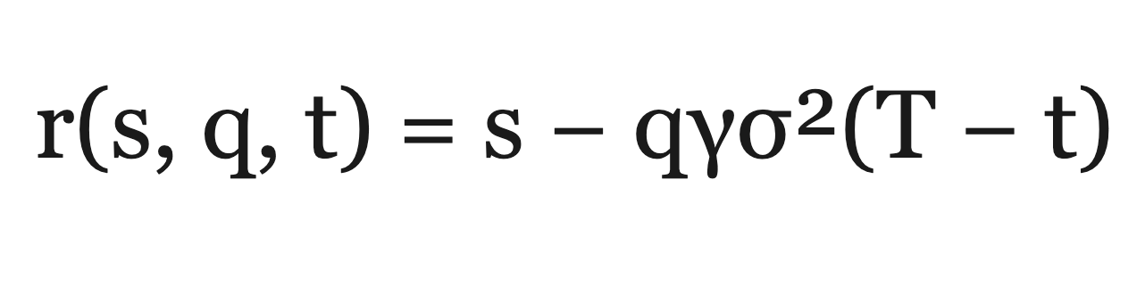
where γ is the dealer’s risk aversion and T − t is the time left in the session. A long position (q > 0) pulls the reservation price below the mid, tilting both quotes down so the dealer is more likely to sell back toward flat. The optimal total spread is

where k governs how quickly fill probability decays with distance from the mid. This is the formula reproduced, with only cosmetic variation, across the current crop of practitioner explainers, including the Hummingbot market-making guide and the HFT Book reference page that calls it “the canonical model for optimal market-making quotes under inventory risk.” Neither site is used below for any figure, only for how the model is currently presented.
The founding paper’s own numbers
Avellaneda and Stoikov tested their inventory strategy against a symmetric benchmark that quotes the identical spread but centers it on the mid-price instead of the reservation price, running 1,000 simulated price paths for three levels of risk aversion (s = 100, T = 1, σ = 2, k = 1.5, A = 140 held fixed throughout). Their published tables give the following mean profit and profit dispersion across those paths.
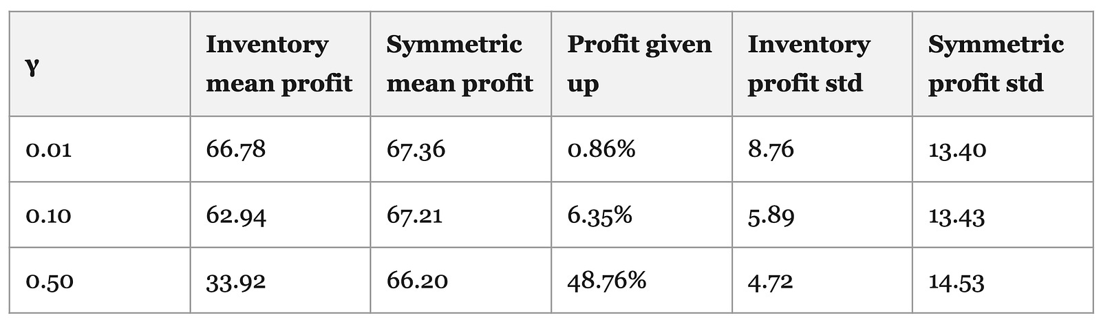
The inventory strategy never wins on mean profit, and that is by design, since it is buying something else: the standard deviation of final inventory fell from 8.66 to 2.80 shares at γ = 0.10 and from 9.06 to 1.88 at γ = 0.50. The symmetric quoter earns more for a mechanical reason. It quotes tighter to the mid on average and fills more often, and when every counterparty is an uninformed Poisson arrival, more fills at a given spread means more expected profit.
The number worth staring at is the jump between rows. The cost of skewing runs 0.86%, then 6.35%, then 48.76%. Dividing each strategy’s mean profit by its own standard deviation, a rough profit-to-dispersion measure that is this piece’s computation and should not be read as an annualized Sharpe ratio, the inventory strategy’s advantage over the symmetric one is 1.52x at γ = 0.01, widens to 2.14x at γ = 0.10, then narrows back to 1.58x at γ = 0.50. Risk-adjusted efficiency peaks in the middle of the tested range. More risk aversion is a better trade than less up to a point, and past that point it is a worse one.
Where the convexity comes from
The acceleration is visible in the spread formula itself. The inventory-risk term γσ²(T − t) scales linearly in γ. The fill-calibration term (2/γ)ln(1 + γ/k) shrinks as γ grows: with the paper’s own k = 1.5, it runs from 1.33 at γ = 0.01 down to 1.15 at γ = 0.50. Avellaneda and Stoikov’s own Tables 1 to 3 report a single “Spread” value per γ, 1.33, 1.29, and 1.15, matching this fill-calibration term exactly; the decomposition below, including the full t = 0 spread in the last column, is this piece’s own computation from the stated formula.
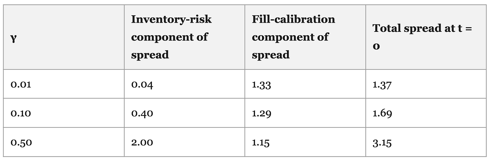
As γ rises, essentially all of the additional spread comes from the inventory-risk term. Because fill intensity decays exponentially with distance from the mid, a spread that widens linearly in γ suppresses the fill rate, and therefore profit, at an accelerating rate. That is the whole mechanism behind the 0.86% to 48.76% jump. It falls directly out of the closed-form solution once its two additive terms are separated, and it means the risk-aversion parameter is a position on a convex cost curve, with an interior optimum that has to be located per instrument, since it moves with σ and k.
There is a second gap between the formula and its own foundations, on timing. Guéant, Lehalle, and Fernandez-Tapia’s 2013 paper solves the same control problem exactly, with a hard inventory limit, and finds the true optimal quotes barely move with time until the session nears its terminal point; the 2008 closed-form quotes are the special case of that exact solution valid only when T − t is small. A formula calibrated, mathematically, for the last stretch of a session is nonetheless what at least some current implementations run across the whole day: the Hummingbot guide linked above implements the plain 2008 formula with no time-independence correction. Whether institutional systems share that pattern is unverifiable from public data, and a 2022 academic study states that extensions in the 2013 lineage are already in use at major market-making firms, so the gap likely sits between open-source tooling and institutional practice rather than inside institutions.
The cost is real in live data too, and it may not be unavoidable
The same 2022 study backtested the model on 30 days of real BTC-USD Level 2 data. A genetically calibrated, static-parameter Avellaneda-Stoikov model produced by far the lowest mean and standard deviation of maximum drawdown among five tested models, while two reinforcement-learning variants that were allowed to deviate from its risk-minimizing quotes beat all three baselines, the pure model included, on Sharpe ratio on 24 of 30 days and Sortino on 25 of 30, at the price of occasional outlier drawdowns. That is the 2008 tradeoff reappearing in live data on the authors’ own reading: a correctly calibrated Avellaneda-Stoikov quote is the risk-minimizing choice by construction, so anything chasing higher risk-adjusted return is accepting more risk somewhere. It is one study, one asset pair, one month, and should be read as a documented data point rather than a settled pattern.
Whether the profit cost is a permanent law of quoting against inventory is a separate and open question. The 2008 model assumes no counterparty knows anything the dealer doesn’t, and early evidence suggests that assumption is what generates the cost: a 2025 preprint by Barzykin, Bergault, Guéant, and Lemmel (not yet peer-reviewed, with one author at HSBC under an HSBC-funded initiative) finds in its numerical illustrations that once order flow is modeled as partly informed, quotes that account for that information can raise expected profit and cut its variance simultaneously relative to informationally naive quoting. If that result survives peer review and replication on live data, the tradeoff documented above is a consequence of one dropped assumption, with a published correction. Until then, it stands as the model’s own arithmetic.
What would change this view
The 0.86%, 6.35%, and 48.76% figures are specific to the paper’s toy parameters (s = 100, σ = 2, k = 1.5, A = 140) and will not reproduce numerically elsewhere. The structural claim generalizes: the cost of risk aversion is convex because one spread component scales linearly in γ while the other shrinks, and that follows from the formula, independent of calibration. What would overturn the practical conclusion is a demonstration that, for realistic calibrations, the interior efficiency peak sits so close to one end of the usable γ range that treating the parameter as a one-directional safety dial loses nothing. The three published points here show a clear interior peak; a denser sweep on a real instrument could in principle show otherwise, and that sweep is exactly the check recommended below.
What to check
Two questions for any system running this model. First, where does the current γ sit on its own cost curve: sweep γ against the desk’s actual σ and k calibration, compute mean profit and its dispersion per setting the way the 2008 paper did, and locate the interior peak instead of assuming more risk aversion is monotonically safer. The founding paper’s own three data points show it is not. Second, is the system running the 2013 exact quotes or the 2008 asymptotic ones, since the latter are accurate only near the session close and the difference is a documented, closed-form correction, published for over a decade. Both checks run in hours against a calibration the desk already owns, and each prices something currently being paid for without being measured.
📊 Want Deeper Quantitative Analysis?
This research took a long stretch of data collection, verification, and analysis. If you found value in this deep-dive, I publish exclusive quantitative research, trading strategies, and institutional-grade analysis on Patreon. By joining, you’ll be supporting my work and motivating me to publish more content like this.
→ Join the Patreon community here
You can also follow my work here:
YouTube: The Mathematical Trader
LinkedIn: Navnoor Bawa
Cover photograph: Joe Mabel, CC BY-SA 3.0, via Wikimedia Commons.