36% Returns: How D.E. Shaw Beat Citadel & Millennium to Top 2024

D.E. Shaw’s Oculus Fund posted 36.1% net returns while Composite delivered 18%, earning $11.1 billion for investors to claim #1 on the 2024 LCH rankings. Here’s the technical breakdown.

---

This is a detailed research piece. If you find value in institutional-quality hedge fund analysis, support this work on Patreon.

D.E. Shaw topped LCH Investments’ 2024 hedge fund rankings with $11.1 billion in net investor gains, beating Millennium ($9.4B) and Citadel ($9.0B). The firm’s Composite Fund returned 18% net while Oculus surged 36.1%, its best year since 2004 inception. Both funds remain closed to new capital, and the firm returned approximately half of 2024 profits to outside investors.

This article deconstructs the mathematical frameworks and P&L engines behind these returns, based on verified public disclosures and industry-standard quantitative methods.

Performance Snapshot

Composite Fund

• 2024 return: 18% net

• Annualized since 2001: 12.7%

• 18 of 23 years with double-digit gains

Oculus Fund

• 2024 return: 36.1% net (record)

• Annualized since 2004: 13.7%

• Reported to have no losing years (not independently verifiable from public NAV history)

Firm-wide

• AUM: $65 billion

• Lifetime investor gains: $67.2 billion (#2 all-time)

• 2024 global rank: #1

Sources: Bloomberg, Hedgeweek, LCH Investments

---

I. Statistical Arbitrage: The Core Engine

Mathematical Framework

D.E. Shaw’s stat arb traces to Morgan Stanley’s APT Group (1985–1989), where David Shaw worked under Nunzio Tartaglia. The group made $50M in 1987 using pairs trading: buying/selling cointegrated stocks when spreads deviate from equilibrium.

Cointegration test:

Spread S(t) = P_A(t) - β × P_B(t)
ADF test: H₀ = unit root (reject if t-stat < -2.86 at 5% level)

Mean reversion model (Ornstein-Uhlenbeck):

dS(t) = θ(μ - S(t))dt + σdW(t)

θ = mean-reversion speed
μ = long-run mean
Half-life = ln(2)/θ

Kalman filter for dynamic hedge ratios:

State: β_t = β_{t-1} + w_t
Observation: y_t = β_t × x_t + v_t
Kalman gain: K_t = P_t|t-1 × x_t / (x_t² × P_t|t-1 + R)

Execution at Scale

• Portfolio: 4,348 equity positions (Q4 2024 13F filing)

• Infrastructure: In-house execution systems and low-latency architecture (the firm publishes limited public detail on exact latency metrics)

• Technology: 700+ developers (firm materials, 2024), proprietary tools

Walk-forward validation prevents overfitting:

1. In-sample (200 days): Optimize parameters
2. Out-of-sample (52 days): Test on unseen data
3. Deploy only if OOS Sharpe > 1.0

Sources: QuantStart, Hudson Thames

---

II. Oculus: Macro Systematic 36.1% Return

2024 Trade Mechanics (Verified)

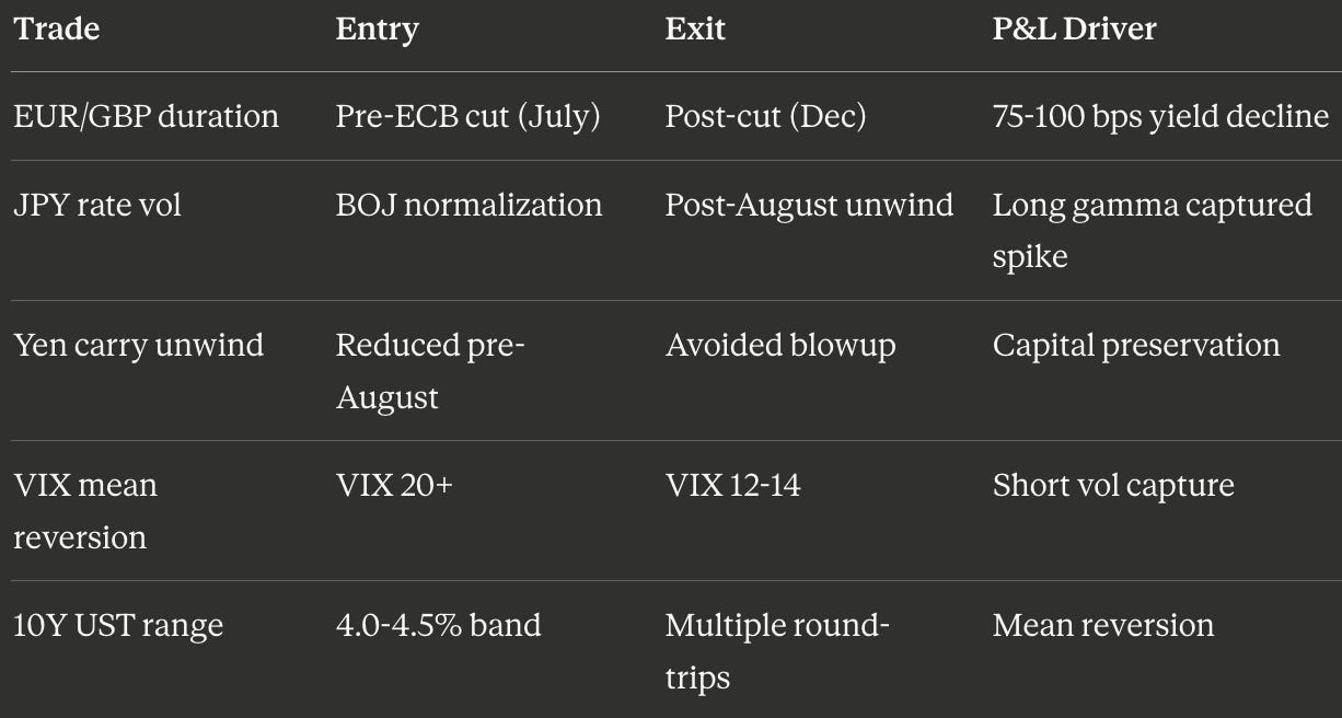
Regime-Switching Framework

Hidden Markov Model for state detection:

States: Low Vol, High Vol, Crisis
Transition matrix determines portfolio allocation

Low Vol → Sell options, carry trades
High Vol → Reduce exposure, long gamma
Crisis → Flight to quality, long vol

Result: Reported to have no losing years in its 20-year history per industry sources, though full NAV history is not publicly available.

Sources: Hedgeweek, Alternative Fund Insight

---

III. Derivatives: Gamma & Volatility Alpha

Convertible Arbitrage P&L

Position structure:

Long: Convertible bond (bond + embedded call)
Short: Δ shares of stock (delta-hedge)

Gamma trading mechanics:

Stock rises $1 → Bond gains more than stock short loses
→ Rehedge: Short more stock at HIGHER price

Stock falls $1 → Bond loses less than stock short gains
→ Rehedge: Cover stock at LOWER price

Net: Buy low, sell high automatically
Gamma P&L ≈ 0.5 × Γ × (ΔS)²

LETF Decay Arbitrage

Why 3x ETFs decay:

Day 1: Index at 100
Day 2: Index +10% → 110
Day 3: Index -9.09% → 100 (flat)

3x LETF:
Day 2: +30% → 130
Day 3: -27.27% → 94.55 (-5.45% vs flat index)

Strategy: Short both 3x Bull and 3x Bear
Capture: Volatility decay from daily rebalancing

Source: Investopedia — Convertible Arbitrage

---

IV. Private Credit: Diopter Synthetic Risk Transfer

Fund Structure

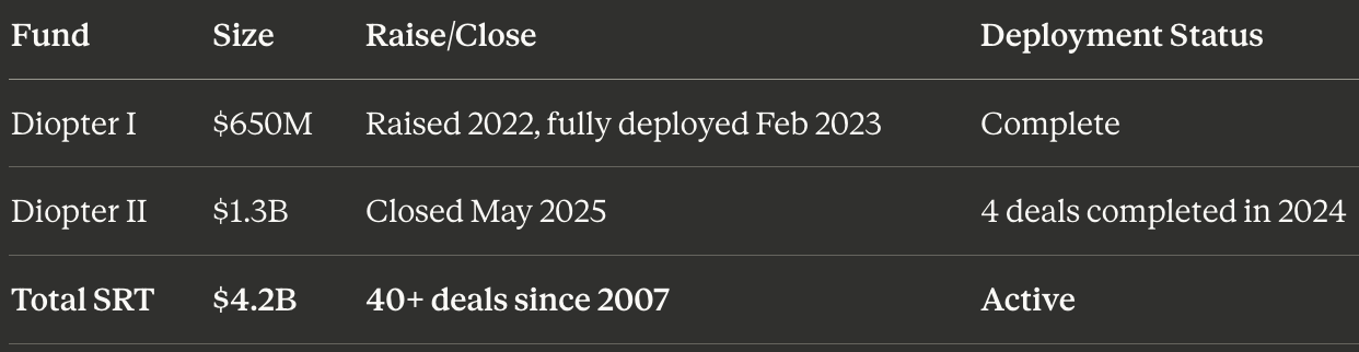
Deal Mechanics

Bank holds $5B loan portfolio
Problem: Consumes $400M regulatory capital (8% RWA)

Solution: Sell first-loss protection to D.E. Shaw
- D.E. Shaw posts $500M collateral (10% first-loss)
- Absorbs first 10% of portfolio losses
- Collects 300-500 bps annual premium

If 0.5% losses ($25M):
Premium collected: ~$150M over 3 years
Net P&L: $125M profit

If 5% losses ($250M):
Loss from collateral: $250M
Net P&L: Negative (tail risk)

Edge: Quant models analyze “blind pools” with limited borrower visibility by cross-referencing loan characteristics with public data.

Sources: Hedgeweek, Institutional Investor, Bloomberg

---

V. Index & ETF Arbitrage

Rebalancing Alpha

S&P 500 addition mechanism:

Day 0: Announcement (stock ABC to be added)
Days 1-4: Index funds must buy → price pressure
Day 5: Effective date (peak demand)
Day 6+: Premium dissipates

Arbitrage:
- Buy on announcement at $50
- Sell into index buying at $55 (10% gain)
- Capture temporary mispricing

D.E. Shaw edge: Predict additions before announcement using constituent rules + market cap monitoring.

ETF Creation/Redemption

When NAV ≠ ETF price:

Premium: Create ETF shares, sell at premium, lock in spread
Discount: Buy ETF shares, redeem for basket, sell securities

Execution speed + scale = profitable even on 5-10 bps mispricings

Source: Investopedia — Index Arbitrage

---

VI. Event-Driven: Merger Arbitrage

Mechanics

Cash deal example:

Acquirer offers $100/share cash
Target trades at $95 (5% spread = deal risk)

Position: Long target at $95
Holding period: 6 months
If deal closes: $5 profit (10.6% annualized)
If deal fails: Drop to $75 (-21% loss)

Risk-adjusted sizing:
P(close) = 85%
Expected return = 0.85 × 5.3% + 0.15 × (-21%) = 1.4%

Stock-for-stock hedge:

Acquirer offers 0.8 shares per target share
Acquirer at $120 → Implied value = $96
Target at $93 → Spread = $3 (3.2%)

Position:
- Long 1 target share at $93
- Short 0.8 acquirer shares at $120

Lock in $3 spread regardless of market moves

Source: D.E. Shaw — What We Do

---

VII. Technology & Execution

Infrastructure

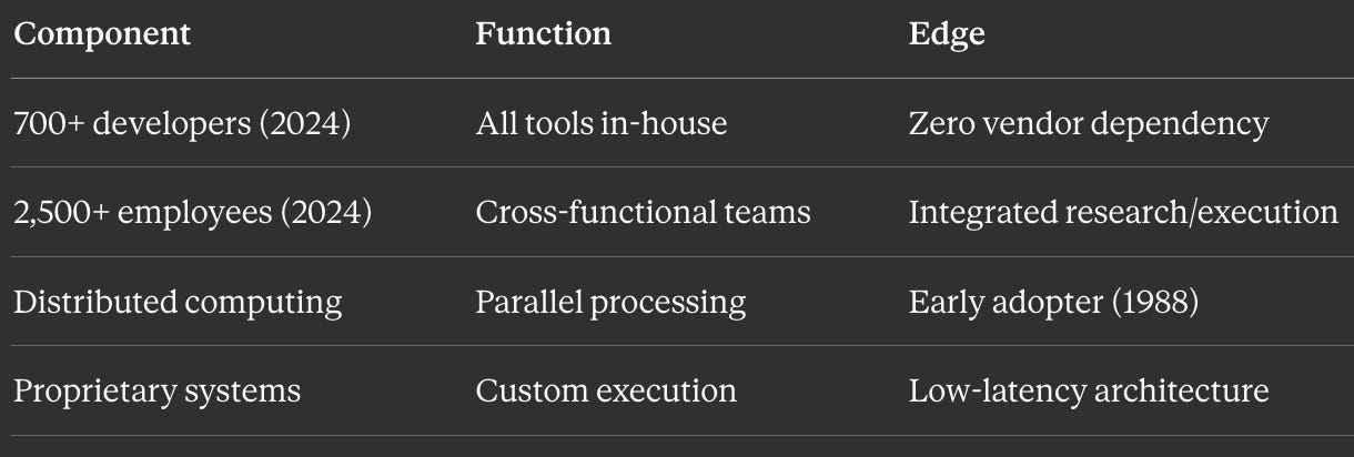
Transaction Cost Optimization

Implementation shortfall minimization:

IS = (Execution Price - Decision Price) × Shares

Components:
- Market impact: f(order size, liquidity, urgency)
- Spread cost: 0.5 × bid-ask × shares
- Timing delay: Price drift during execution
- Opportunity cost: Missed trades

At scale: A one-basis-point improvement can translate into tens of millions of dollars annually

Source: D.E. Shaw GitHub

---

VIII. Risk Management & Portfolio Construction

Position Sizing: Fractional Kelly

Formula:

f* = (p × b - q) / b
Fractional: f = 0.25-0.5 × f*

Rationale: Full Kelly too aggressive
Fractional reduces variance with minimal growth sacrifice

Multi-Strategy Allocation (Illustrative)

Composite Fund breakdown:
├── Equity Stat Arb: 25-35%
├── Systematic Macro: 15-25%
├── Discretionary Credit: 10-20%
├── Convertible/Options: 5-15%
├── Event-Driven: 5-15%
├── Energy: 3-8%
├── Reinsurance/ILS: 2-5%
└── Private Credit: 3-8%

Risk attribution:

• VaR (1-day, 10-day tail risk)

• Stress tests: 2008, COVID, rate shocks

• Factor exposure: Market, size, value, momentum

• Real-time P&L attribution by strategy

Official stance: “Every one of us is a risk manager. Portfolio and risk management are not separated.”

Source: D.E. Shaw Risk Management PDF

---

IX. Fee Economics & Capital Discipline

Fee Structure (Industry Sources)

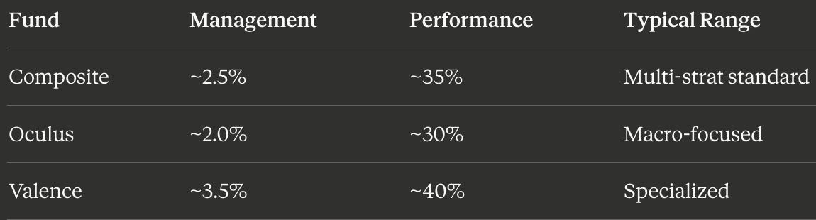
Capital Discipline

2024 action: Returned ~50% of Composite + Oculus profits to investors despite record performance.

Rationale:

More capital → Higher market impact → Lower returns
Optimal AUM = argmax(Fee revenue × Sustainable Sharpe)

Historical precedent: Both flagship funds closed to new capital in early 2020s. In 2023, returned all profits to investors despite single-digit gains.

Result: Lifetime gains ($67.2B) exceed current AUM ($65B), proof of disciplined capital management.

Sources: Institutional Investor, Alternative Fund Insight

---

The Competitive Moat

1. Intellectual Capital

• PhD-heavy research teams (physicists, mathematicians, computer scientists)

• 700+ developers building proprietary systems (firm materials, 2024)

• Continuous ML/AI innovation on ghost patterns

2. Execution Infrastructure

• Proprietary execution systems built in-house

• Direct market access across all asset classes

• Low-latency architecture optimized for speed

3. Diversification

• 10+ uncorrelated P&L engines

• Systematic + discretionary + hybrid strategies

• Public + private markets exposure

4. Capital Discipline

• Closed to new capital when optimal

• Return profits to maintain capacity

• Reject growth that dilutes alpha

5. Track Record

• Composite: 12.7% annualized (23 years)

• Oculus: 13.7% annualized (20 years, reported to have no losing years)

• $67.2B lifetime investor gains (#2 all-time)

---

Key Takeaways

1. Mathematical rigor: OU processes, Kalman filters, regime-switching models (not discretionary intuition)

2. Walk-forward validation: Prevents overfitting, ensures out-of-sample performance

3. Scale + speed: 4,348 positions (Q4 2024 13F), proprietary infrastructure, optimized execution

4. Diversification: 10 distinct engines with low cross-correlation

5. Capacity discipline: Return capital rather than dilute alpha

6. Hybrid model: Systematic + discretionary + ML-driven signals

2024 Result: $11.1B investor gains, 18% Composite, 36.1% Oculus (#1 globally).

---

Verified Sources

Performance & Rankings

• Institutional Investor — LCH Rankings

• Bloomberg — 2024 Returns

• Hedgeweek — Performance Analysis

• Alternative Fund Insight

Diopter & Private Credit

• Hedgeweek — Diopter II

• Institutional Investor — Diopter Strategy

• Bloomberg — Blind Pools

Historical & Technical

• Institutional Investor — APT Group Origins

• Hudson Thames — Pairs Trading History

• QuantStart — Kalman Filter

• SEC 13F Filings — D.E. Shaw Holdings

• D.E. Shaw Official

• D.E. Shaw Risk Management

Academic & Industry

• Investopedia — Convertible Arbitrage

• Investopedia — Index Arbitrage

• Wikipedia — Ornstein-Uhlenbeck Process

• Wikipedia — Kelly Criterion

---

Data verified through December 31, 2025. Performance figures are net returns per LCH Investments rankings. Holdings data from SEC Form 13F filings (Q4 2024). Mathematical frameworks reflect industry-standard implementations documented in academic literature and open-source quantitative finance resources.

📊 Support this research: https://www.patreon.com/c/NavnoorBawa

Cover photograph: Ajay Suresh, CC BY 4.0, via Wikimedia Commons.